Drawing vector maps with simple features and ggplot2
library(tidyverse)
library(sf)
library(here)

options(digits = 3)
set.seed(1234)
theme_set(theme_minimal())
Unlike raster image maps, vector maps require you to obtain spatial data files which contain detailed information necessary to draw all the components of a map (e.g. points, lines, polygons). Once you successfully import that data into R, ggplot2 works with simple features data frames to easily generate geospatial visualizations using all the core elements and approaches of ggplot().
Import USA state boundaries
First we will import a spatial data file containing the boundaries of all 50 states in the United States1 using sf::st_read():
usa <- here(
  "static", "data", "census_bureau",
  "cb_2013_us_state_20m", "cb_2013_us_state_20m.shp"
) %>%
  st_read()
## Reading layer `cb_2013_us_state_20m' from data source `/Users/soltoffbc/Projects/Computing for Social Sciences/course-site/static/data/census_bureau/cb_2013_us_state_20m/cb_2013_us_state_20m.shp' using driver `ESRI Shapefile'
## Simple feature collection with 52 features and 9 fields
## Geometry type: MULTIPOLYGON
## Dimension:     XY
## Bounding box:  xmin: -179 ymin: 17.9 xmax: 180 ymax: 71.4
## Geodetic CRS:  NAD83
Draw the boundaries
ggplot2 contains a geometric object specifically for simple feature objects called geom_sf(). This works reasonably well when you need to draw polygons, like our state boundaries. Support for simple features in ggplot2 is under active development, so you may not find adequate support for plotting line or point features. To draw the map, we pass the simple features data frame as the data argument.
ggplot(data = usa) +
  geom_sf()
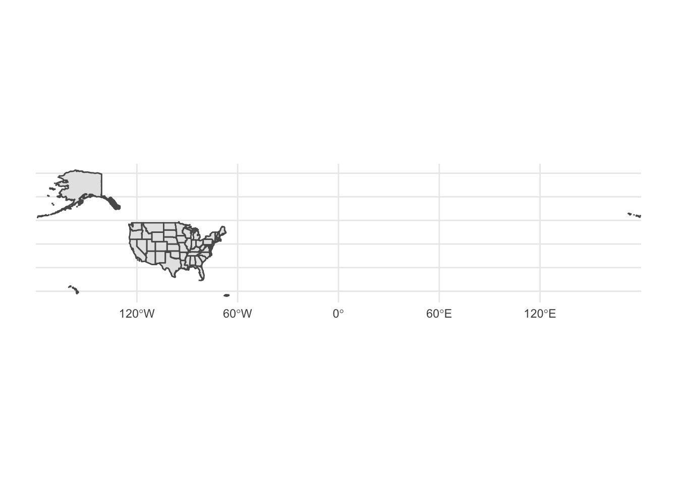
Because simple features data frames are standardized with the geometry column always containing information on the geographic coordinates of the features, we do not need to specify additional parameters for aes(). Notice a problem with the map above: it wastes a lot of space. This is caused by the presence of Alaska and Hawaii in the dataset. The Aleutian Islands cross the the 180th meridian, requiring the map to show the Eastern hemisphere. Likewise, Hawaii is substantially distant from the continental United States.
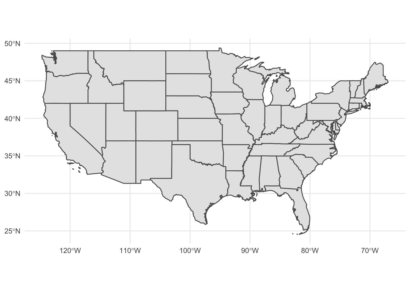
Plot a subset of a map
One solution is to plot just the lower 48 states. That is, exclude Alaska and Hawaii, as well as DC and Puerto Rico.2 Because simple features data frames contain one row per feature and in this example a feature is defined as a state, we can use filter() from dplyr to exclude these four states/territories.
(usa_48 <- usa %>%
  filter(!(NAME %in% c("Alaska", "District of Columbia", "Hawaii", "Puerto Rico"))))
## Simple feature collection with 48 features and 9 fields
## geometry type:  MULTIPOLYGON
## dimension:      XY
## bbox:           xmin: -125 ymin: 24.5 xmax: -66.9 ymax: 49.4
## geographic CRS: NAD83
## First 10 features:
##    STATEFP  STATENS    AFFGEOID GEOID STUSPS        NAME LSAD    ALAND   AWATER
## 1       01 01779775 0400000US01    01     AL     Alabama   00 1.31e+11 4.59e+09
## 2       05 00068085 0400000US05    05     AR    Arkansas   00 1.35e+11 2.96e+09
## 3       06 01779778 0400000US06    06     CA  California   00 4.03e+11 2.05e+10
## 4       09 01779780 0400000US09    09     CT Connecticut   00 1.25e+10 1.82e+09
## 5       12 00294478 0400000US12    12     FL     Florida   00 1.39e+11 3.14e+10
## 6       13 01705317 0400000US13    13     GA     Georgia   00 1.49e+11 4.95e+09
## 7       16 01779783 0400000US16    16     ID       Idaho   00 2.14e+11 2.40e+09
## 8       17 01779784 0400000US17    17     IL    Illinois   00 1.44e+11 6.20e+09
## 9       18 00448508 0400000US18    18     IN     Indiana   00 9.28e+10 1.54e+09
## 10      20 00481813 0400000US20    20     KS      Kansas   00 2.12e+11 1.35e+09
##                          geometry
## 1  MULTIPOLYGON (((-88.3 30.2,...
## 2  MULTIPOLYGON (((-94.6 36.5,...
## 3  MULTIPOLYGON (((-119 33.5, ...
## 4  MULTIPOLYGON (((-73.7 41.1,...
## 5  MULTIPOLYGON (((-80.7 24.9,...
## 6  MULTIPOLYGON (((-85.6 35, -...
## 7  MULTIPOLYGON (((-117 44.4, ...
## 8  MULTIPOLYGON (((-91.5 40.2,...
## 9  MULTIPOLYGON (((-88.1 37.9,...
## 10 MULTIPOLYGON (((-102 40, -1...
ggplot(data = usa_48) +
  geom_sf()
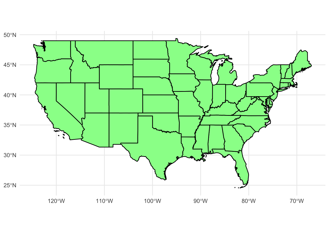
Since the map is a ggplot() object, it can easily be modified like any other ggplot() graph. We could change the color of the map and the borders:
ggplot(data = usa_48) +
  geom_sf(fill = "palegreen", color = "black")
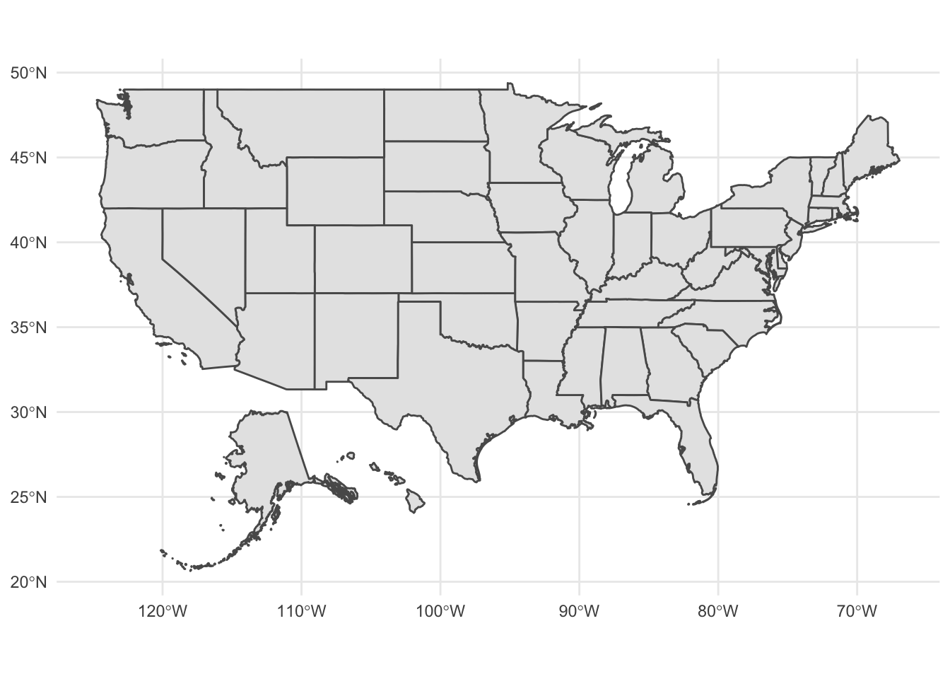
albersusa
Rather than excluding them entirely, most maps of the United States place Alaska and Hawaii as insets to the south of California. Until recently, in R this was an extremely tedious task that required manually changing the latitude and longitude coordinates for these states to place them in the correct location. Fortunately several packages are now available that have already done the work for you. albersusa includes the usa_sf() function which returns a simple features data frame which contains adjusted coordinates for Alaska and Hawaii to plot them with the mainland. It can be installed from GitHub using devtools::install_github("hrbrmstr/albersusa").
library(albersusa)
usa_sf()
## Simple feature collection with 51 features and 13 fields
## geometry type:  MULTIPOLYGON
## dimension:      XY
## bbox:           xmin: -125 ymin: 20.6 xmax: -66.9 ymax: 49.4
## geographic CRS: WGS 84
## First 10 features:
##         geo_id fips_state                 name lsad census_area iso_3166_2
## 1  0400000US04         04              Arizona           113594         AZ
## 2  0400000US05         05             Arkansas            52035         AR
## 3  0400000US06         06           California           155779         CA
## 4  0400000US08         08             Colorado           103642         CO
## 5  0400000US09         09          Connecticut             4842         CT
## 6  0400000US11         11 District of Columbia               61         DC
## 7  0400000US13         13              Georgia            57513         GA
## 8  0400000US17         17             Illinois            55519         IL
## 9  0400000US18         18              Indiana            35826         IN
## 10 0400000US22         22            Louisiana            43204         LA
##      census pop_estimataes_base pop_2010 pop_2011 pop_2012 pop_2013 pop_2014
## 1   6392017             6392310  6411999  6472867  6556236  6634997  6731484
## 2   2915918             2915958  2922297  2938430  2949300  2958765  2966369
## 3  37253956            37254503 37336011 37701901 38062780 38431393 38802500
## 4   5029196             5029324  5048575  5119661  5191709  5272086  5355866
## 5   3574097             3574096  3579345  3590537  3594362  3599341  3596677
## 6    601723              601767   605210   620427   635040   649111   658893
## 7   9687653             9688681  9714464  9813201  9919000  9994759 10097343
## 8  12830632            12831587 12840097 12858725 12873763 12890552 12880580
## 9   6483802             6484192  6490308  6516560  6537632  6570713  6596855
## 10  4533372             4533479  4545581  4575972  4604744  4629284  4649676
##                          geometry
## 1  MULTIPOLYGON (((-113 37, -1...
## 2  MULTIPOLYGON (((-94 33, -94...
## 3  MULTIPOLYGON (((-120 34, -1...
## 4  MULTIPOLYGON (((-107 41, -1...
## 5  MULTIPOLYGON (((-72.4 42, -...
## 6  MULTIPOLYGON (((-77 38.8, -...
## 7  MULTIPOLYGON (((-84.8 35, -...
## 8  MULTIPOLYGON (((-89.4 42.5,...
## 9  MULTIPOLYGON (((-84.8 40.4,...
## 10 MULTIPOLYGON (((-88.9 29.8,...
ggplot(data = usa_sf()) +
  geom_sf()
Add data to the map
Region boundaries serve as the background in geospatial data visualization - so now we need to add data. Some types of geographic data (points and symbols) are overlaid on top of the boundaries, whereas other data (fill) are incorporated into the region layer itself.
Points
Let’s use our usa_48 map data to add some points. The airports data frame in the nycflights13 package includes geographic info on airports in the United States.
library(nycflights13)
airports
## # A tibble: 1,458 x 8
##    faa   name                       lat    lon   alt    tz dst   tzone
##    <chr> <chr>                    <dbl>  <dbl> <dbl> <dbl> <chr> <chr>
##  1 04G   Lansdowne Airport         41.1  -80.6  1044    -5 A     America/New_Yo…
##  2 06A   Moton Field Municipal A…  32.5  -85.7   264    -6 A     America/Chicago
##  3 06C   Schaumburg Regional       42.0  -88.1   801    -6 A     America/Chicago
##  4 06N   Randall Airport           41.4  -74.4   523    -5 A     America/New_Yo…
##  5 09J   Jekyll Island Airport     31.1  -81.4    11    -5 A     America/New_Yo…
##  6 0A9   Elizabethton Municipal …  36.4  -82.2  1593    -5 A     America/New_Yo…
##  7 0G6   Williams County Airport   41.5  -84.5   730    -5 A     America/New_Yo…
##  8 0G7   Finger Lakes Regional A…  42.9  -76.8   492    -5 A     America/New_Yo…
##  9 0P2   Shoestring Aviation Air…  39.8  -76.6  1000    -5 U     America/New_Yo…
## 10 0S9   Jefferson County Intl     48.1 -123.    108    -8 A     America/Los_An…
## # … with 1,448 more rows
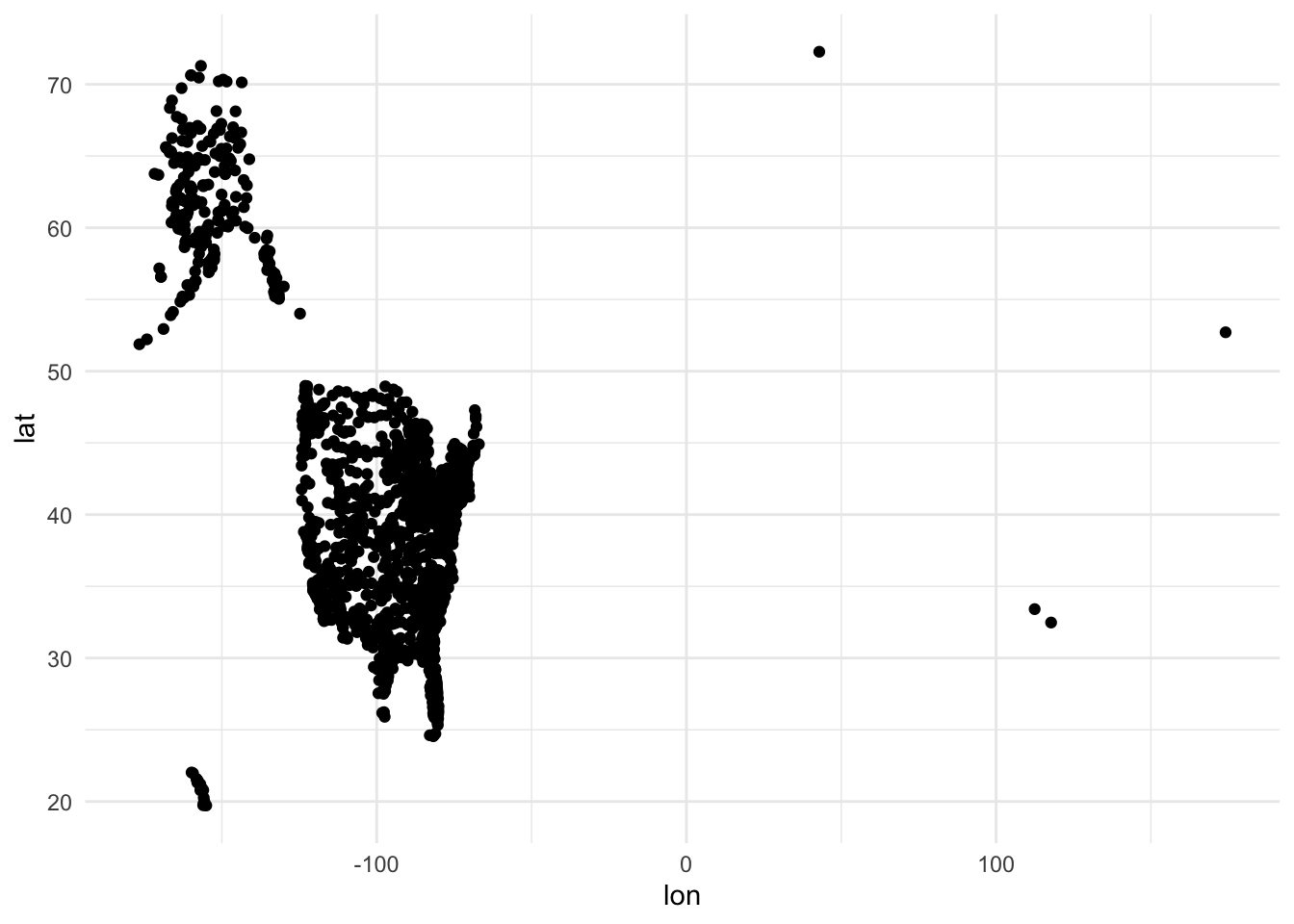
Each airport has it’s geographic location encoded through lat and lon. To draw these points on the map, basically we draw a scatterplot with x = lon and y = lat. In fact we could simply do that:
ggplot(airports, aes(lon, lat)) +
  geom_point()
Let’s overlay it with the mapped state borders:
ggplot(data = usa_48) +
  geom_sf() +
  geom_point(data = airports, aes(x = lon, y = lat), shape = 1)
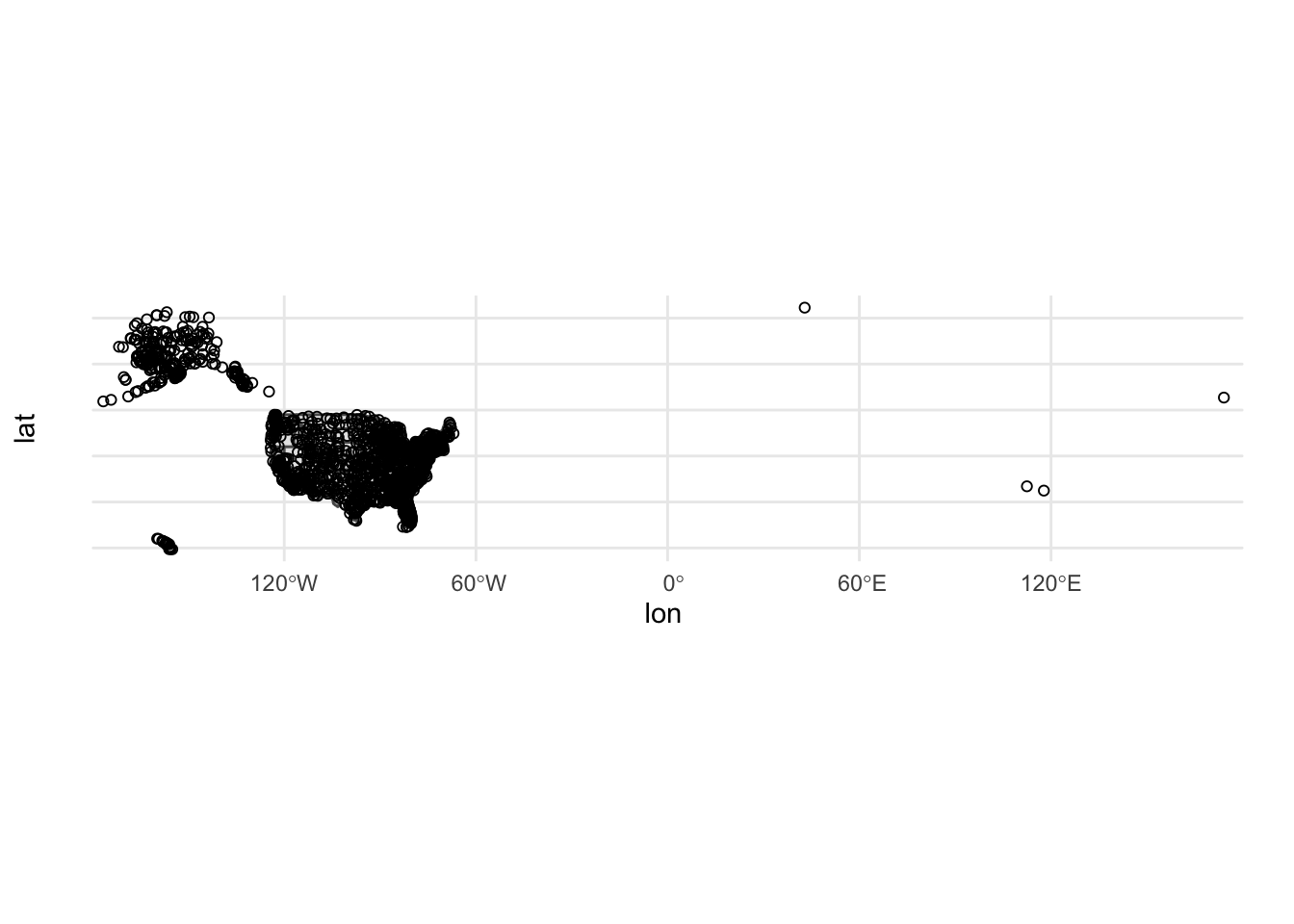
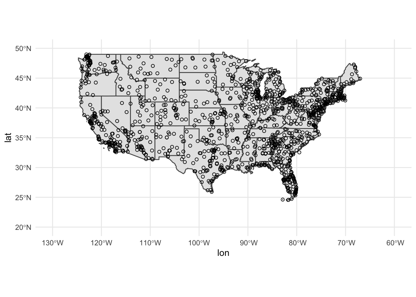
Slight problem. We have airports listed outside of the continental United States. There are a couple ways to rectify this. Unfortunately airports does not include a variable identifying state so the filter() operation is not that simple. The easiest solution is to crop the limits of the graph using coord_sf() to only show the mainland:
ggplot(data = usa_48) +
  geom_sf() +
  geom_point(data = airports, aes(x = lon, y = lat), shape = 1) +
  coord_sf(
    xlim = c(-130, -60),
    ylim = c(20, 50)
  )
Alternatively, we can use st_as_sf() to convert airports to a simple features data frame.
airports_sf <- st_as_sf(airports, coords = c("lon", "lat"))
st_crs(airports_sf) <- 4326 # set the coordinate reference system
airports_sf
## Simple feature collection with 1458 features and 6 fields
## Geometry type: POINT
## Dimension:     XY
## Bounding box:  xmin: -177 ymin: 19.7 xmax: 174 ymax: 72.3
## Geodetic CRS:  WGS 84
## # A tibble: 1,458 x 7
##    faa   name                    alt    tz dst   tzone                  geometry
##  * <chr> <chr>                 <dbl> <dbl> <chr> <chr>               <POINT [°]>
##  1 04G   Lansdowne Airport      1044    -5 A     America/New_…      (-80.6 41.1)
##  2 06A   Moton Field Municipa…   264    -6 A     America/Chic…      (-85.7 32.5)
##  3 06C   Schaumburg Regional     801    -6 A     America/Chic…        (-88.1 42)
##  4 06N   Randall Airport         523    -5 A     America/New_…      (-74.4 41.4)
##  5 09J   Jekyll Island Airport    11    -5 A     America/New_…      (-81.4 31.1)
##  6 0A9   Elizabethton Municip…  1593    -5 A     America/New_…      (-82.2 36.4)
##  7 0G6   Williams County Airp…   730    -5 A     America/New_…      (-84.5 41.5)
##  8 0G7   Finger Lakes Regiona…   492    -5 A     America/New_…      (-76.8 42.9)
##  9 0P2   Shoestring Aviation …  1000    -5 U     America/New_…      (-76.6 39.8)
## 10 0S9   Jefferson County Intl   108    -8 A     America/Los_…       (-123 48.1)
## # … with 1,448 more rows
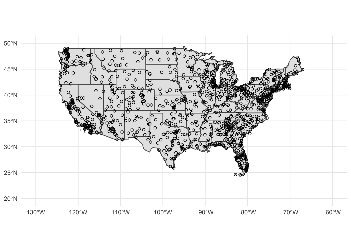
coords tells st_as_sf() which columns contain the geographic coordinates of each airport. To graph the points on the map, we use a second geom_sf():
ggplot() +
  geom_sf(data = usa_48) +
  geom_sf(data = airports_sf, shape = 1) +
  coord_sf(
    xlim = c(-130, -60),
    ylim = c(20, 50)
  )
Symbols
We can change the size or type of symbols on the map. For instance, we can draw a bubble plot (also known as a proportional symbol map) and encode the altitude of the airport through the size channel:
ggplot(data = usa_48) +
  geom_sf() +
  geom_point(
    data = airports, aes(x = lon, y = lat, size = alt),
    fill = "grey", color = "black", alpha = .2
  ) +
  coord_sf(
    xlim = c(-130, -60),
    ylim = c(20, 50)
  ) +
  scale_size_area(guide = FALSE)
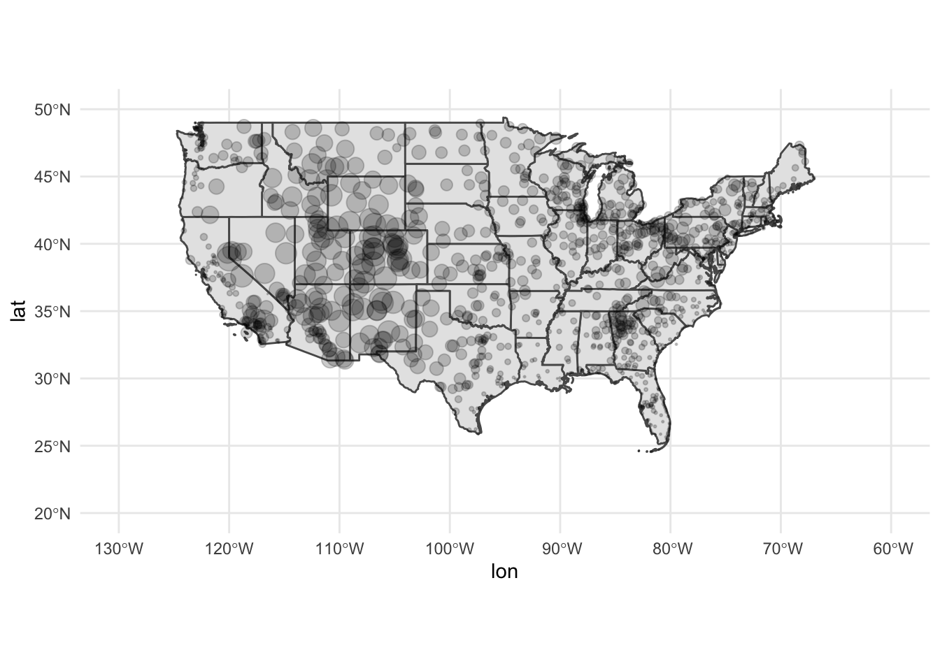
Circle area is proportional to the airport’s altitude (in feet). Or we could scale it based on the number of arriving flights in flights:
airports_n <- flights %>%
  count(dest) %>%
  left_join(airports, by = c("dest" = "faa"))

ggplot(data = usa_48) +
  geom_sf() +
  geom_point(
    data = airports_n, aes(x = lon, y = lat, size = n),
    fill = "grey", color = "black", alpha = .2
  ) +
  coord_sf(
    xlim = c(-130, -60),
    ylim = c(20, 50)
  ) +
  scale_size_area(guide = FALSE)
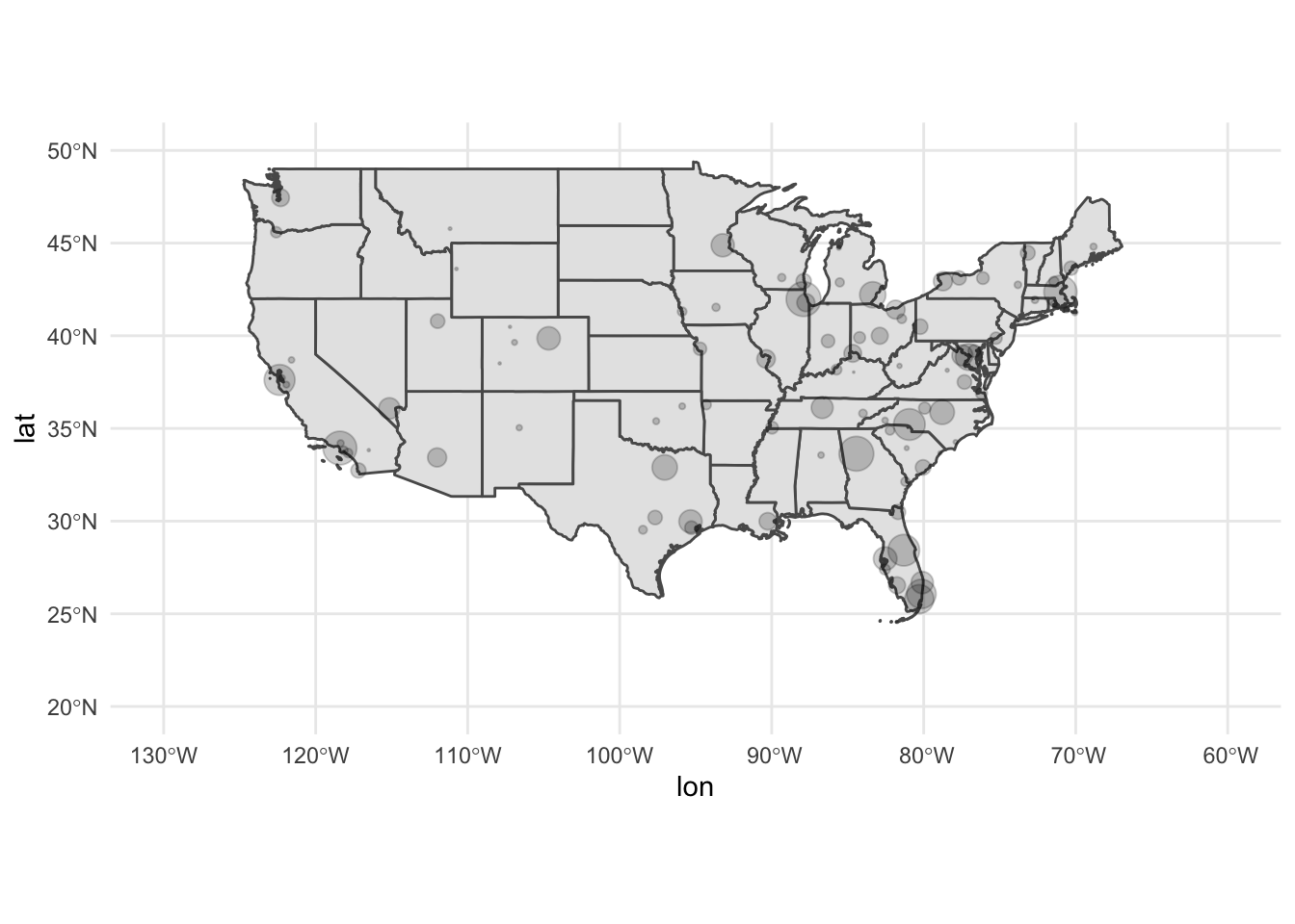
airports contains a list of virtually all commercial airports in the United States. However flights only contains data on flights departing from New York City airports (JFK, LaGuardia, or Newark) and only services a few airports around the country.Fill (choropleths)
Choropleth maps encode information by assigning shades of colors to defined areas on a map (e.g. countries, states, counties, zip codes). There are lots of ways to tweak and customize these graphs, which is generally a good idea because remember that color is one of the harder-to-decode channels.
We will continue to use the usa_48 simple features data frame and draw a choropleth for the number of foreign-born individuals in each state. We get those files from the census_bureau folder. Let’s also normalize our measure by the total population to get the rate of foreign-born individuals in the population:
(fb_state <- here(
  "static", "data", "census_bureau",
  "ACS_13_5YR_B05012_state", "ACS_13_5YR_B05012.csv"
) %>%
  read_csv() %>%
  mutate(rate = HD01_VD03 / HD01_VD01))
## # A tibble: 51 x 10
##    GEO.id     GEO.id2 `GEO.display-labe… HD01_VD01 HD02_VD01 HD01_VD02 HD02_VD02
##    <chr>      <chr>   <chr>                  <dbl> <lgl>         <dbl>     <dbl>
##  1 0400000US… 01      Alabama              4799277 NA          4631045      2881
##  2 0400000US… 02      Alaska                720316 NA           669941      1262
##  3 0400000US… 04      Arizona              6479703 NA          5609835      7725
##  4 0400000US… 05      Arkansas             2933369 NA          2799972      2568
##  5 0400000US… 06      California          37659181 NA         27483342     30666
##  6 0400000US… 08      Colorado             5119329 NA          4623809      5778
##  7 0400000US… 09      Connecticut          3583561 NA          3096374      5553
##  8 0400000US… 10      Delaware              908446 NA           831683      2039
##  9 0400000US… 11      District of Colum…    619371 NA           534142      2017
## 10 0400000US… 12      Florida             19091156 NA         15392410     16848
## # … with 41 more rows, and 3 more variables: HD01_VD03 <dbl>, HD02_VD03 <dbl>,
## #   rate <dbl>
Join the data
Now that we have our data, we want to draw it on the map. fb_state contains one row per state, as does usa_48. Since there is a one-to-one match between the data frames, we join the data frames together first, then use that single data frame to draw the map. This differs from the approach above for drawing points because a point feature is not the same thing as a polygon feature. That is, there were more airports then there were states. Because the spatial data is stored in a data frame with one row per state, all we need to do is merge the data frames together on a column that uniquely identifies each row in each data frame.
(usa_fb <- usa_48 %>%
  left_join(fb_state, by = c("STATEFP" = "GEO.id2")))
## Simple feature collection with 48 features and 18 fields
## geometry type:  MULTIPOLYGON
## dimension:      XY
## bbox:           xmin: -125 ymin: 24.5 xmax: -66.9 ymax: 49.4
## geographic CRS: NAD83
## First 10 features:
##    STATEFP  STATENS    AFFGEOID GEOID STUSPS        NAME LSAD    ALAND   AWATER
## 1       01 01779775 0400000US01    01     AL     Alabama   00 1.31e+11 4.59e+09
## 2       05 00068085 0400000US05    05     AR    Arkansas   00 1.35e+11 2.96e+09
## 3       06 01779778 0400000US06    06     CA  California   00 4.03e+11 2.05e+10
## 4       09 01779780 0400000US09    09     CT Connecticut   00 1.25e+10 1.82e+09
## 5       12 00294478 0400000US12    12     FL     Florida   00 1.39e+11 3.14e+10
## 6       13 01705317 0400000US13    13     GA     Georgia   00 1.49e+11 4.95e+09
## 7       16 01779783 0400000US16    16     ID       Idaho   00 2.14e+11 2.40e+09
## 8       17 01779784 0400000US17    17     IL    Illinois   00 1.44e+11 6.20e+09
## 9       18 00448508 0400000US18    18     IN     Indiana   00 9.28e+10 1.54e+09
## 10      20 00481813 0400000US20    20     KS      Kansas   00 2.12e+11 1.35e+09
##         GEO.id GEO.display-label HD01_VD01 HD02_VD01 HD01_VD02 HD02_VD02
## 1  0400000US01           Alabama   4799277        NA   4631045      2881
## 2  0400000US05          Arkansas   2933369        NA   2799972      2568
## 3  0400000US06        California  37659181        NA  27483342     30666
## 4  0400000US09       Connecticut   3583561        NA   3096374      5553
## 5  0400000US12           Florida  19091156        NA  15392410     16848
## 6  0400000US13           Georgia   9810417        NA   8859747      7988
## 7  0400000US16             Idaho   1583364        NA   1489560      2528
## 8  0400000US17          Illinois  12848554        NA  11073828     10091
## 9  0400000US18           Indiana   6514861        NA   6206801      4499
## 10 0400000US20            Kansas   2868107        NA   2677007      3095
##    HD01_VD03 HD02_VD03   rate                       geometry
## 1     168232      2881 0.0351 MULTIPOLYGON (((-88.3 30.2,...
## 2     133397      2568 0.0455 MULTIPOLYGON (((-94.6 36.5,...
## 3   10175839     30666 0.2702 MULTIPOLYGON (((-119 33.5, ...
## 4     487187      5553 0.1360 MULTIPOLYGON (((-73.7 41.1,...
## 5    3698746     16848 0.1937 MULTIPOLYGON (((-80.7 24.9,...
## 6     950670      7988 0.0969 MULTIPOLYGON (((-85.6 35, -...
## 7      93804      2528 0.0592 MULTIPOLYGON (((-117 44.4, ...
## 8    1774726     10093 0.1381 MULTIPOLYGON (((-91.5 40.2,...
## 9     308060      4500 0.0473 MULTIPOLYGON (((-88.1 37.9,...
## 10    191100      3100 0.0666 MULTIPOLYGON (((-102 40, -1...
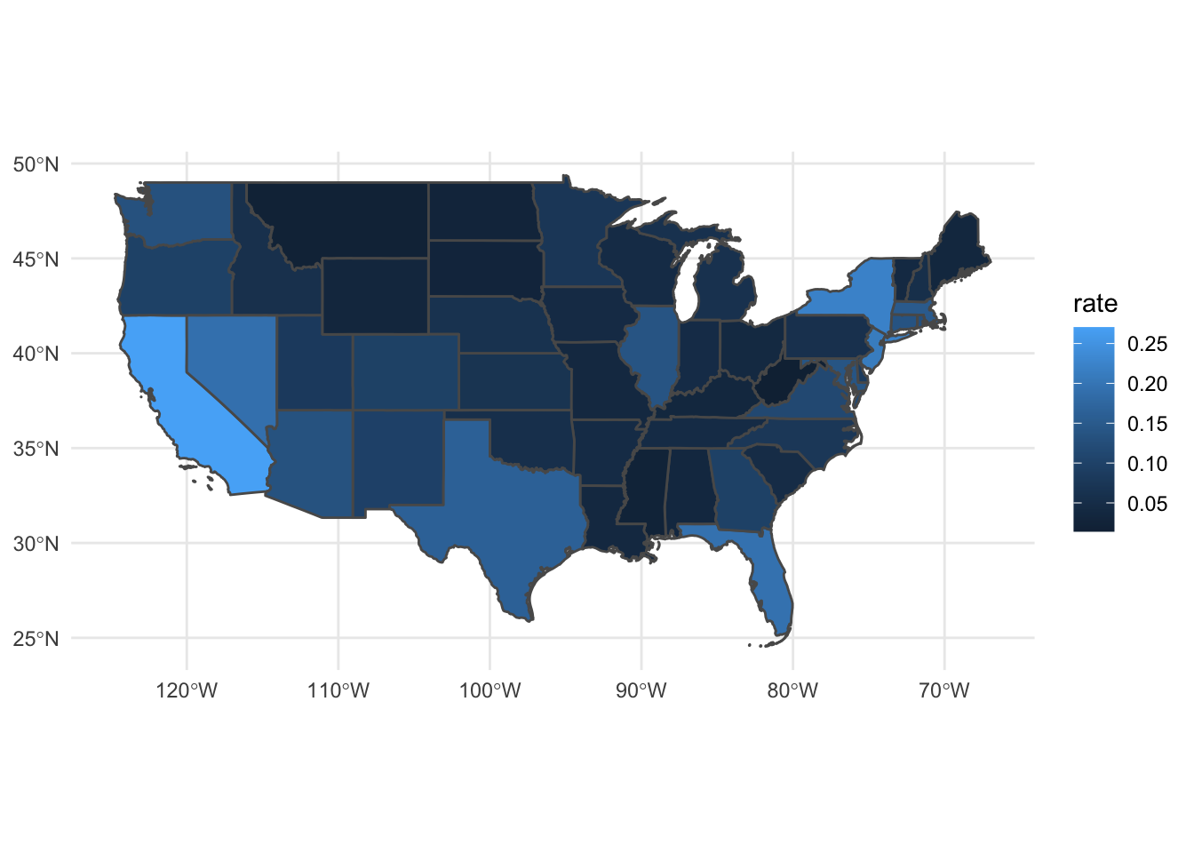
Draw the map
With the newly combined data frame, use geom_sf() and define the fill aesthetic based on the column in usa_fb you want to visualize.
ggplot(data = usa_fb) +
  geom_sf(aes(fill = rate))
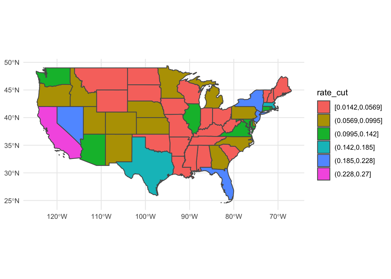
Bin data to discrete intervals
When creating a heatmap with a continuous variable, one must decide whether to keep the variable as continuous or collapse it into a series of bins with discrete colors. While keep the variable continuous is technically more precise, the human eye cannot usually distinguish between two colors which are very similar to one another. By converting the variable to a discrete variable, you easily distinguish between the different levels. If you decide to convert a continuous variable to a discrete variable, you will need to decide how to do this. While cut() is a base R function for converting continuous variables into discrete values, ggplot2 offers two functions that explicitly define how we want to bin the numeric vector (column).
cut_interval() makes n groups with equal range:
usa_fb %>%
  mutate(rate_cut = cut_interval(rate, n = 6)) %>%
  ggplot() +
  geom_sf(aes(fill = rate_cut))
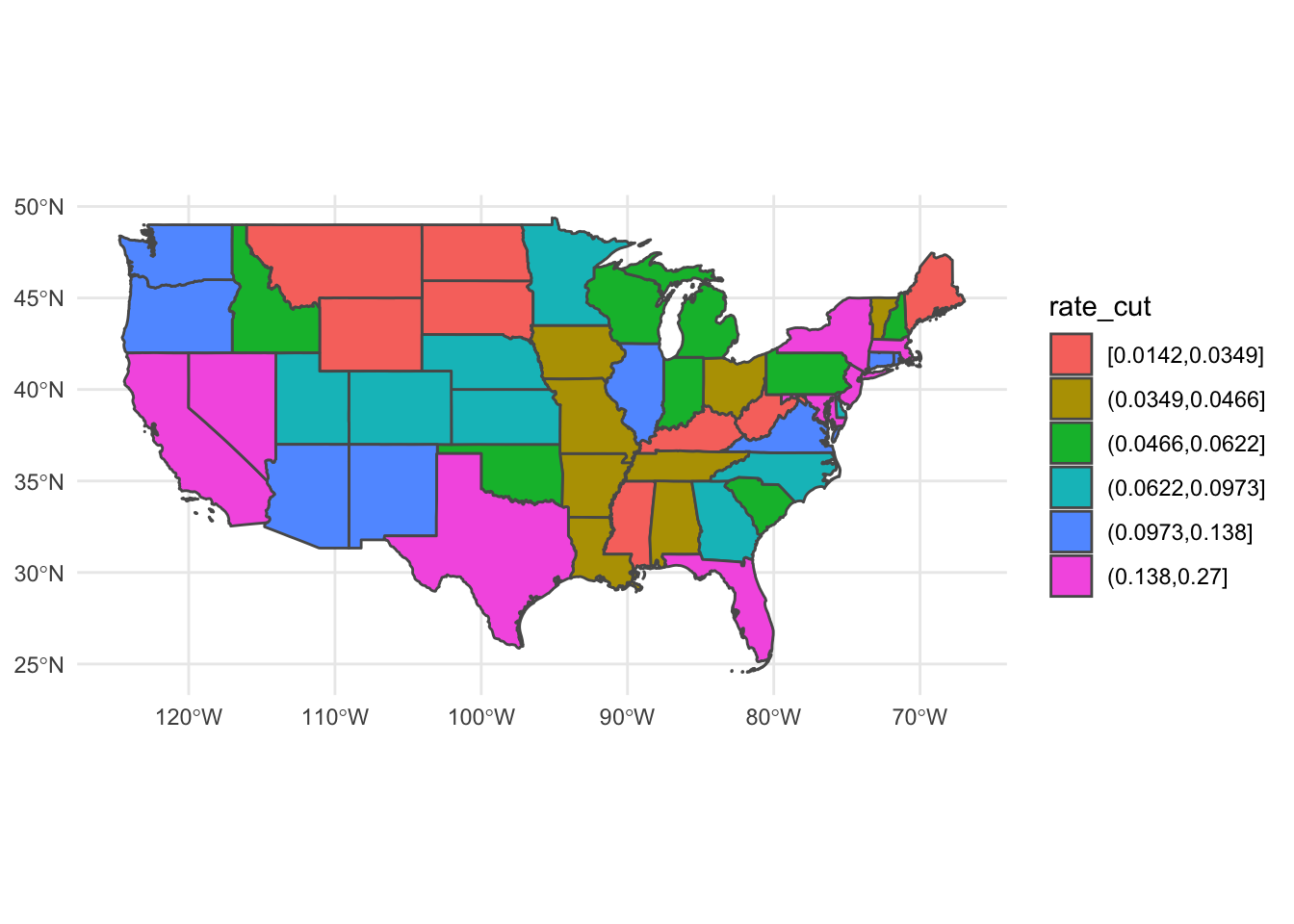
Whereas cut_number() makes n groups with (approximately) equal numbers of observations:
usa_fb %>%
  mutate(rate_cut = cut_number(rate, n = 6)) %>%
  ggplot() +
  geom_sf(aes(fill = rate_cut))
cut_interval() or cut_number().Changing map projection
](https://imgs.xkcd.com/comics/mercator_projection.png)
Representing portions of the globe on a flat surface can be challenging. Depending on how you project the map, you can distort or emphasize certain features of the map. Fortunately, ggplot() includes the coord_sf() function which allows us to easily implement different projection methods. In order to implement coordinate transformations, you need to know the coordinate reference system that defines the projection method. The “easiest” approach is to provide what is known as the proj4string that defines the projection method. PROJ4 is a generic coordinate transformation software that allows you to convert between projection methods. If you get really into geospatial analysis and visualization, it is helpful to learn this system.
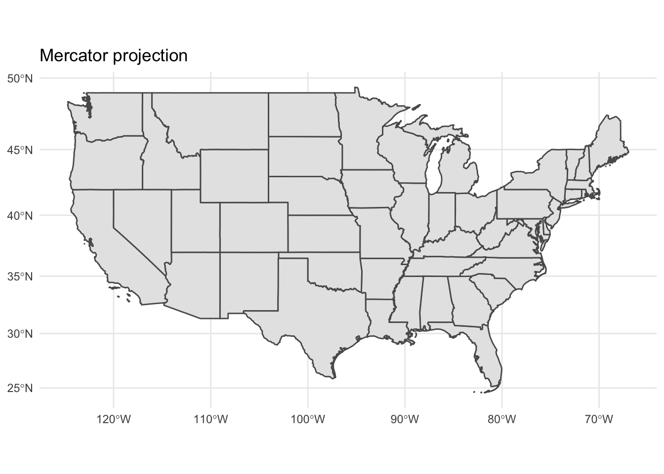
For our purposes here, proj4string is a character string in R that defines the coordinate system and includes parameters specific to a given coordinate transformation. PROJ4 includes some documentation on common projection methods that can get you started. Some projection methods are relatively simple and require just the name of the projection, like for a Mercator projection ("+proj=merc"):
map_proj_base <- ggplot(data = usa_48) +
  geom_sf()
map_proj_base +
  coord_sf(crs = "+proj=merc") +
  ggtitle("Mercator projection")
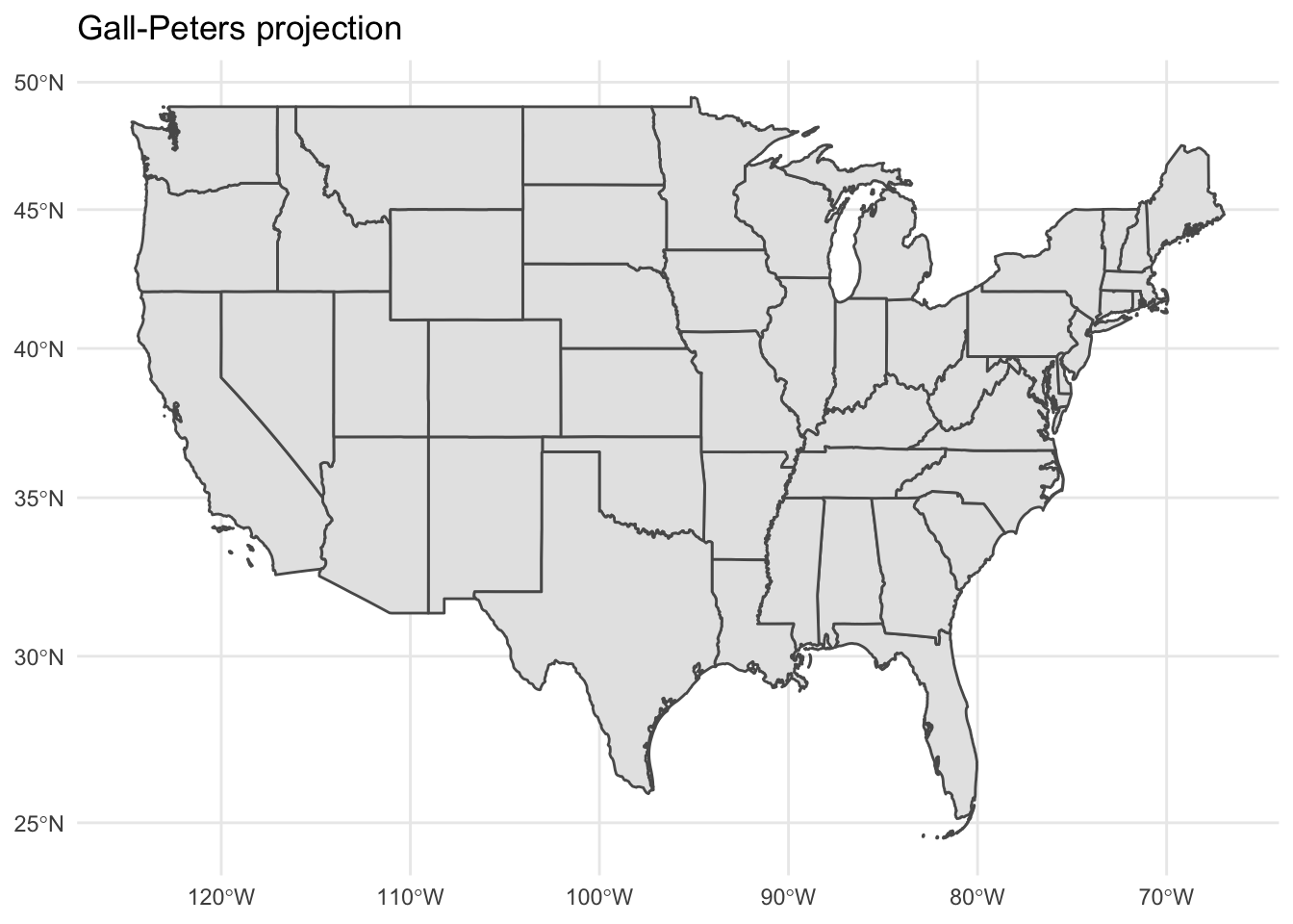
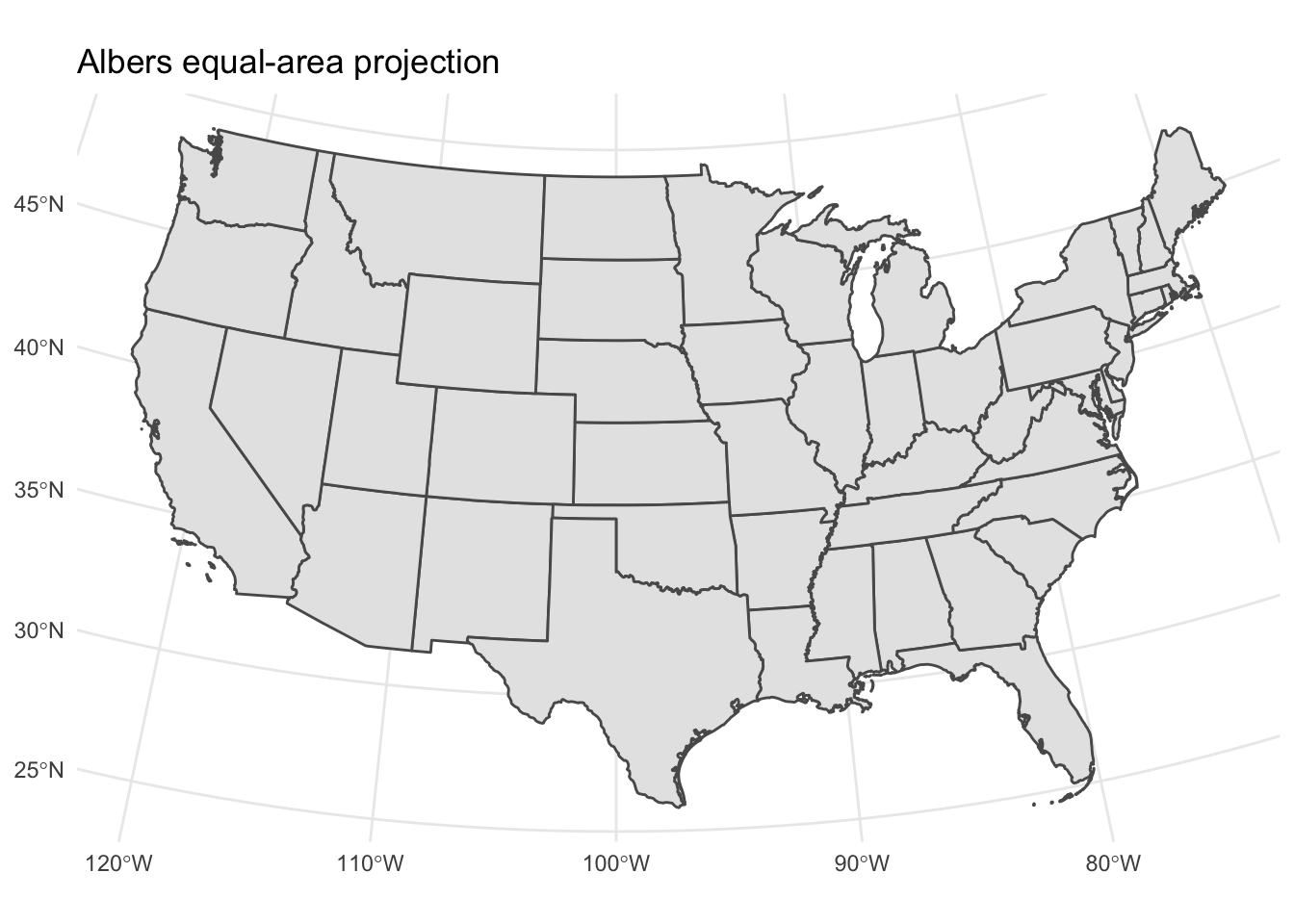
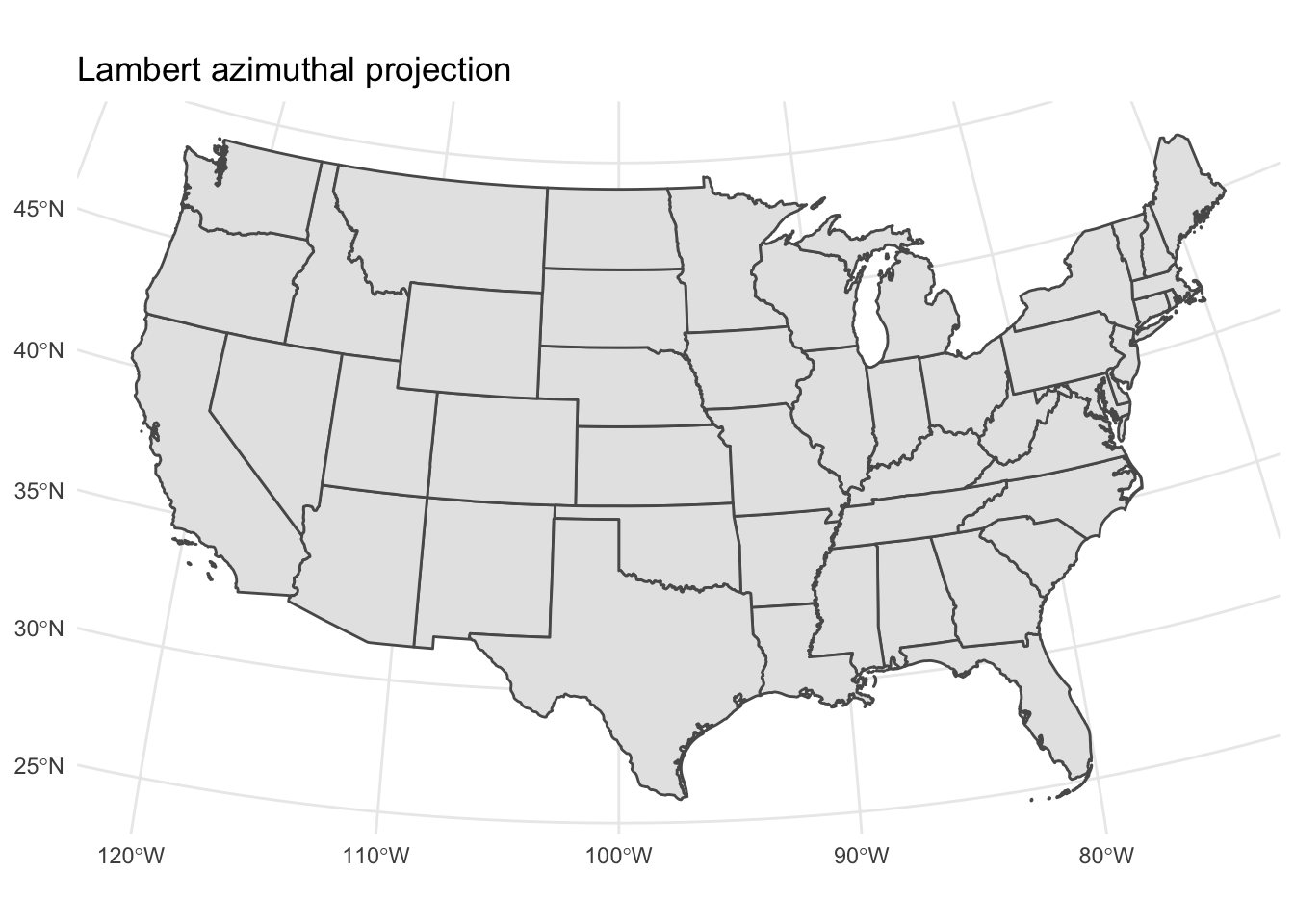
Other coordinate systems require specification of the standard lines, or lines that define areas of the surface of the map that are tangent to the globe. These include Gall-Peters, Albers equal-area, and Lambert azimuthal.
map_proj_base +
  coord_sf(crs = "+proj=cea +lon_0=0 +lat_ts=45") +
  ggtitle("Gall-Peters projection")
map_proj_base +
  coord_sf(crs = "+proj=aea +lat_1=25 +lat_2=50 +lon_0=-100") +
  ggtitle("Albers equal-area projection")
map_proj_base +
  coord_sf(crs = "+proj=laea +lat_0=35 +lon_0=-100") +
  ggtitle("Lambert azimuthal projection")
Session Info
devtools::session_info()
## ─ Session info ───────────────────────────────────────────────────────────────
##  setting  value
##  version  R version 4.0.4 (2021-02-15)
##  os       macOS Big Sur 10.16
##  system   x86_64, darwin17.0
##  ui       X11
##  language (EN)
##  collate  en_US.UTF-8
##  ctype    en_US.UTF-8
##  tz       America/Chicago
##  date     2021-07-13
##
## ─ Packages ───────────────────────────────────────────────────────────────────
##  package     * version date       lib source
##  assertthat    0.2.1   2019-03-21 [2] CRAN (R 4.0.0)
##  backports     1.2.1   2020-12-09 [2] CRAN (R 4.0.2)
##  blogdown      1.3     2021-04-14 [2] CRAN (R 4.0.2)
##  bookdown      0.22    2021-04-22 [2] CRAN (R 4.0.2)
##  broom         0.7.6   2021-04-05 [2] CRAN (R 4.0.4)
##  bslib         0.2.5   2021-05-12 [2] CRAN (R 4.0.4)
##  cachem        1.0.5   2021-05-15 [2] CRAN (R 4.0.2)
##  callr         3.7.0   2021-04-20 [2] CRAN (R 4.0.2)
##  cellranger    1.1.0   2016-07-27 [2] CRAN (R 4.0.0)
##  class         7.3-19  2021-05-03 [2] CRAN (R 4.0.2)
##  classInt      0.4-3   2020-04-07 [2] CRAN (R 4.0.0)
##  cli           2.5.0   2021-04-26 [2] CRAN (R 4.0.2)
##  colorspace    2.0-1   2021-05-04 [2] CRAN (R 4.0.2)
##  crayon        1.4.1   2021-02-08 [2] CRAN (R 4.0.2)
##  DBI           1.1.1   2021-01-15 [2] CRAN (R 4.0.2)
##  dbplyr        2.1.1   2021-04-06 [2] CRAN (R 4.0.4)
##  desc          1.3.0   2021-03-05 [2] CRAN (R 4.0.2)
##  devtools      2.4.1   2021-05-05 [2] CRAN (R 4.0.2)
##  digest        0.6.27  2020-10-24 [2] CRAN (R 4.0.2)
##  dplyr       * 1.0.6   2021-05-05 [2] CRAN (R 4.0.2)
##  e1071         1.7-6   2021-03-18 [2] CRAN (R 4.0.2)
##  ellipsis      0.3.2   2021-04-29 [2] CRAN (R 4.0.2)
##  evaluate      0.14    2019-05-28 [2] CRAN (R 4.0.0)
##  fansi         0.4.2   2021-01-15 [2] CRAN (R 4.0.2)
##  fastmap       1.1.0   2021-01-25 [2] CRAN (R 4.0.2)
##  forcats     * 0.5.1   2021-01-27 [2] CRAN (R 4.0.2)
##  fs            1.5.0   2020-07-31 [2] CRAN (R 4.0.2)
##  generics      0.1.0   2020-10-31 [2] CRAN (R 4.0.2)
##  ggplot2     * 3.3.3   2020-12-30 [2] CRAN (R 4.0.2)
##  glue          1.4.2   2020-08-27 [2] CRAN (R 4.0.2)
##  gtable        0.3.0   2019-03-25 [2] CRAN (R 4.0.0)
##  haven         2.4.1   2021-04-23 [2] CRAN (R 4.0.2)
##  here        * 1.0.1   2020-12-13 [2] CRAN (R 4.0.2)
##  hms           1.1.0   2021-05-17 [2] CRAN (R 4.0.4)
##  htmltools     0.5.1.1 2021-01-22 [2] CRAN (R 4.0.2)
##  httr          1.4.2   2020-07-20 [2] CRAN (R 4.0.2)
##  jquerylib     0.1.4   2021-04-26 [2] CRAN (R 4.0.2)
##  jsonlite      1.7.2   2020-12-09 [2] CRAN (R 4.0.2)
##  KernSmooth    2.23-20 2021-05-03 [2] CRAN (R 4.0.2)
##  knitr         1.33    2021-04-24 [2] CRAN (R 4.0.2)
##  lifecycle     1.0.0   2021-02-15 [2] CRAN (R 4.0.2)
##  lubridate     1.7.10  2021-02-26 [2] CRAN (R 4.0.2)
##  magrittr      2.0.1   2020-11-17 [2] CRAN (R 4.0.2)
##  memoise       2.0.0   2021-01-26 [2] CRAN (R 4.0.2)
##  modelr        0.1.8   2020-05-19 [2] CRAN (R 4.0.0)
##  munsell       0.5.0   2018-06-12 [2] CRAN (R 4.0.0)
##  pillar        1.6.1   2021-05-16 [2] CRAN (R 4.0.4)
##  pkgbuild      1.2.0   2020-12-15 [2] CRAN (R 4.0.2)
##  pkgconfig     2.0.3   2019-09-22 [2] CRAN (R 4.0.0)
##  pkgload       1.2.1   2021-04-06 [2] CRAN (R 4.0.2)
##  prettyunits   1.1.1   2020-01-24 [2] CRAN (R 4.0.0)
##  processx      3.5.2   2021-04-30 [2] CRAN (R 4.0.2)
##  proxy         0.4-25  2021-03-05 [2] CRAN (R 4.0.2)
##  ps            1.6.0   2021-02-28 [2] CRAN (R 4.0.2)
##  purrr       * 0.3.4   2020-04-17 [2] CRAN (R 4.0.0)
##  R6            2.5.0   2020-10-28 [2] CRAN (R 4.0.2)
##  Rcpp          1.0.6   2021-01-15 [2] CRAN (R 4.0.2)
##  readr       * 1.4.0   2020-10-05 [2] CRAN (R 4.0.2)
##  readxl        1.3.1   2019-03-13 [2] CRAN (R 4.0.0)
##  remotes       2.3.0   2021-04-01 [2] CRAN (R 4.0.2)
##  reprex        2.0.0   2021-04-02 [2] CRAN (R 4.0.2)
##  rlang         0.4.11  2021-04-30 [2] CRAN (R 4.0.2)
##  rmarkdown     2.8     2021-05-07 [2] CRAN (R 4.0.2)
##  rprojroot     2.0.2   2020-11-15 [2] CRAN (R 4.0.2)
##  rstudioapi    0.13    2020-11-12 [2] CRAN (R 4.0.2)
##  rvest         1.0.0   2021-03-09 [2] CRAN (R 4.0.2)
##  sass          0.4.0   2021-05-12 [2] CRAN (R 4.0.2)
##  scales        1.1.1   2020-05-11 [2] CRAN (R 4.0.0)
##  sessioninfo   1.1.1   2018-11-05 [2] CRAN (R 4.0.0)
##  sf          * 0.9-8   2021-03-17 [2] CRAN (R 4.0.2)
##  stringi       1.6.1   2021-05-10 [2] CRAN (R 4.0.2)
##  stringr     * 1.4.0   2019-02-10 [2] CRAN (R 4.0.0)
##  testthat      3.0.2   2021-02-14 [2] CRAN (R 4.0.2)
##  tibble      * 3.1.1   2021-04-18 [2] CRAN (R 4.0.2)
##  tidyr       * 1.1.3   2021-03-03 [2] CRAN (R 4.0.2)
##  tidyselect    1.1.1   2021-04-30 [2] CRAN (R 4.0.2)
##  tidyverse   * 1.3.1   2021-04-15 [2] CRAN (R 4.0.2)
##  units         0.7-1   2021-03-16 [2] CRAN (R 4.0.2)
##  usethis       2.0.1   2021-02-10 [2] CRAN (R 4.0.2)
##  utf8          1.2.1   2021-03-12 [2] CRAN (R 4.0.2)
##  vctrs         0.3.8   2021-04-29 [2] CRAN (R 4.0.2)
##  withr         2.4.2   2021-04-18 [2] CRAN (R 4.0.2)
##  xfun          0.23    2021-05-15 [2] CRAN (R 4.0.2)
##  xml2          1.3.2   2020-04-23 [2] CRAN (R 4.0.0)
##  yaml          2.2.1   2020-02-01 [2] CRAN (R 4.0.0)
##
## [1] /Users/soltoffbc/Library/R/4.0/library
## [2] /Library/Frameworks/R.framework/Versions/4.0/Resources/library