Iteration

library(tidyverse)
library(rcfss)
library(palmerpenguins)

set.seed(1234)
theme_set(theme_minimal())

Run the code below in your console to download this exercise as a set of R scripts.

usethis::use_course("uc-cfss/vectors-and-iteration")

Writing `for` loops

Functions are one method of reducing duplication in your code. Another tool for reducing duplication is iteration, which lets you do the same thing to multiple inputs.

Example `for` loop

df <- tibble(
  a = rnorm(10),
  b = rnorm(10),
  c = rnorm(10),
  d = rnorm(10)
)

Let’s say we want to compute the median for each column.

median(df$a)

## [1] -0.5555419

median(df$b)

## [1] -0.4941011

median(df$c)

## [1] -0.4656169

median(df$d)

## [1] -0.605349

Boo! We’ve copied-and-pasted median() three times. We don’t want to do that. Instead, we can use a for loop:

output <- vector(mode = "double", length = ncol(df))
for (i in seq_along(df)) {
  output[[i]] <- median(df[[i]])
}
output

## [1] -0.5555419 -0.4941011 -0.4656169 -0.6053490

Let’s review the three components of every for loop.

Output

output <- vector("double", length = ncol(df))

Before you start a loop, you need to create an empty vector to store the output of the loop. Preallocating space for your output is much more efficient than creating space as you move through the loop. The vector() function allows you to create an empty vector of any type. The first argument mode defines the type of vector (“logical”, “integer”, “double”, “character”, etc.) and the second argument length defines the length of the vector.

Numeric vectors are initialized to 0, logical vectors are initialized to FALSE, character vectors are initialized to "", and list elements to NULL.

vector(mode = "double", length = ncol(df))

## [1] 0 0 0 0

vector(mode = "logical", length = ncol(df))

## [1] FALSE FALSE FALSE FALSE

vector(mode = "character", length = ncol(df))

## [1] "" "" "" ""

vector(mode = "list", length = ncol(df))

## [[1]]
## NULL
## 
## [[2]]
## NULL
## 
## [[3]]
## NULL
## 
## [[4]]
## NULL

Sequence

i in seq_along(df)

This component determines what to loop over. During each iteration through the for loop, a new value will be assigned to i based on the the defined sequence. Here, the sequence is seq_along(df) which creates a numeric vector for a sequence of numbers beginning at 1 and continuing until it reaches the length of df (the length here is the number of columns in df).

seq_along(df)

## [1] 1 2 3 4

Body

output[[i]] <- median(df[[i]])

This is the code that actually performs the desired calculations. It runs multiple times for every value of i. We use [[ notation to reference each column of df and store it in the appropriate element in output.

Why we preallocate space for the output

If you don’t preallocate space for the output, each time the for loop iterates, it makes a copy of the output and appends the new value at the end. Copying data takes time and memory. If the output is preallocated space, the loop simply fills in the slots with the correct values.

Consider the following task: duplicate the data frame palmerpenguins::penguins 100 times and bind them together into a single data frame. We can accomplish the latter task using bind_rows(), and use a for loop to create 100 copies of penguins. What is the difference if we preallocate space for the output as opposed to just copying and extending the data frame each time?

# no preallocation
penguins_no_preall <- tibble()

for(i in 1:100){
  penguins_no_preall <- bind_rows(penguins_no_preall, penguins)
}

# with preallocation using a list
penguins_preall <- vector(mode = "list", length = 100)

for(i in 1:100){
  penguins_preall[[i]] <- penguins
}

penguins_preall <- bind_rows(penguins_preall)

Let’s compare the time it takes to complete each of these loops by replicating each example 100 times and measuring how long it takes for the expression to evaluate.

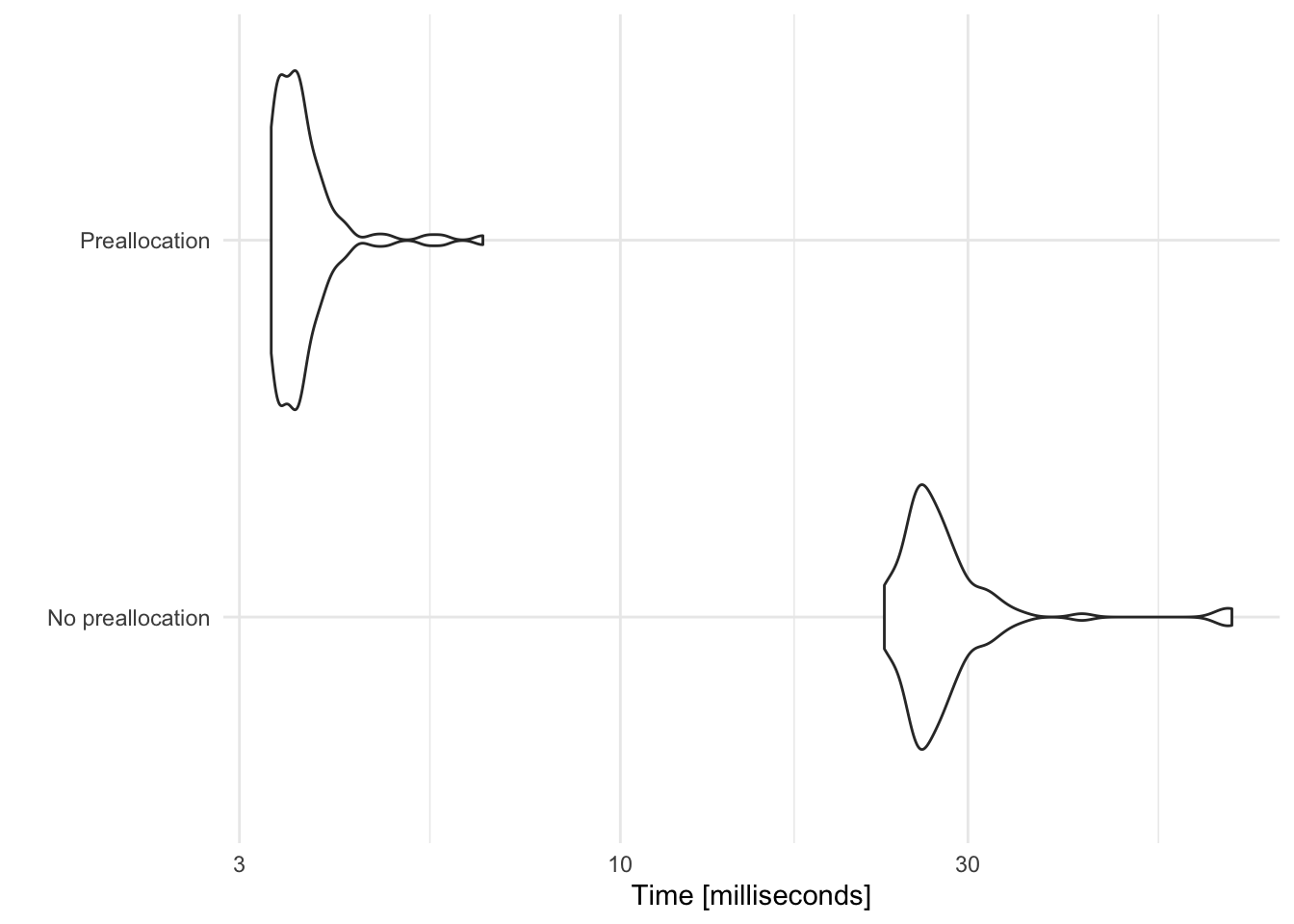
Here, preallocating space for each data frame prior to binding together cuts the computation time by a factor of 10.

Exercise: write a `for` loop

Mean of columns in `mtcars`

Write a for loop that calculates the arithmetic mean for every column in mtcars.

as_tibble(mtcars)

## # A tibble: 32 x 11
##      mpg   cyl  disp    hp  drat    wt  qsec    vs    am  gear  carb
##    <dbl> <dbl> <dbl> <dbl> <dbl> <dbl> <dbl> <dbl> <dbl> <dbl> <dbl>
##  1  21       6  160    110  3.9   2.62  16.5     0     1     4     4
##  2  21       6  160    110  3.9   2.88  17.0     0     1     4     4
##  3  22.8     4  108     93  3.85  2.32  18.6     1     1     4     1
##  4  21.4     6  258    110  3.08  3.22  19.4     1     0     3     1
##  5  18.7     8  360    175  3.15  3.44  17.0     0     0     3     2
##  6  18.1     6  225    105  2.76  3.46  20.2     1     0     3     1
##  7  14.3     8  360    245  3.21  3.57  15.8     0     0     3     4
##  8  24.4     4  147.    62  3.69  3.19  20       1     0     4     2
##  9  22.8     4  141.    95  3.92  3.15  22.9     1     0     4     2
## 10  19.2     6  168.   123  3.92  3.44  18.3     1     0     4     4
## # … with 22 more rows

Before you write the for loop, identify the three components you need:

Output
Sequence
Body

Click for the solution

Output - a numeric vector of length 11
Sequence - i in seq_along(mtcars)

Body - calculate the mean() of the $i$th column, store the new value as the $i$th element of the vector output

# preallocate space for the output
output <- vector("numeric", ncol(mtcars))

# initialize the loop along all the columns of mtcars
for (i in seq_along(mtcars)) {
# calculate the mean value for the i-th column
output[[i]] <- mean(mtcars[[i]], na.rm = TRUE)
}

output

##  [1]  20.090625   6.187500 230.721875 146.687500   3.596563   3.217250
##  [7]  17.848750   0.437500   0.406250   3.687500   2.812500

Maximum value in each column of `diamonds`

Write a for loop that calculates the maximum value in each column of diamonds.

diamonds

## # A tibble: 53,940 x 10
##    carat cut       color clarity depth table price     x     y     z
##    <dbl> <ord>     <ord> <ord>   <dbl> <dbl> <int> <dbl> <dbl> <dbl>
##  1 0.23  Ideal     E     SI2      61.5    55   326  3.95  3.98  2.43
##  2 0.21  Premium   E     SI1      59.8    61   326  3.89  3.84  2.31
##  3 0.23  Good      E     VS1      56.9    65   327  4.05  4.07  2.31
##  4 0.290 Premium   I     VS2      62.4    58   334  4.2   4.23  2.63
##  5 0.31  Good      J     SI2      63.3    58   335  4.34  4.35  2.75
##  6 0.24  Very Good J     VVS2     62.8    57   336  3.94  3.96  2.48
##  7 0.24  Very Good I     VVS1     62.3    57   336  3.95  3.98  2.47
##  8 0.26  Very Good H     SI1      61.9    55   337  4.07  4.11  2.53
##  9 0.22  Fair      E     VS2      65.1    61   337  3.87  3.78  2.49
## 10 0.23  Very Good H     VS1      59.4    61   338  4     4.05  2.39
## # … with 53,930 more rows

Before you write the for loop, identify the three components you need:

Output
Sequence
Body

Click for the solution

Output - a vector of length 10
Sequence - i in seq_along(diamonds)

Body - get the maximum value of the $i$th column of the data frame diamonds, store the new value as the $i$th element of the list output

# preallocate space for the output
output <- vector("numeric", ncol(diamonds))

# initialize the loop along all the columns of diamonds
for (i in seq_along(diamonds)) {
# calculate the max value for the i-th column
output[i] <- max(diamonds[[i]])
}

output

##  [1]     5.01     5.00     7.00     8.00    79.00    95.00 18823.00    10.74
##  [9]    58.90    31.80

To preserve the name attributes from diamonds, use the names() function to extract the names of each column in diamonds and apply them as the names to the output vector:

# get the names of the columns in diamonds
names(diamonds)

##  [1] "carat"   "cut"     "color"   "clarity" "depth"   "table"   "price"  
##  [8] "x"       "y"       "z"

# assign the names of the diamonds columns to output
names(output) <- names(diamonds)
output

##    carat      cut    color  clarity    depth    table    price        x 
##     5.01     5.00     7.00     8.00    79.00    95.00 18823.00    10.74 
##        y        z 
##    58.90    31.80

Notice that all the columns have a maximum value, even the apparently text-based columns. This is because cut, color, and clarity are all stored as factor columns. Remember that factor vectors are built on top of integers, so the underlying values are numeric. As a result we can apply max() to a factor vector and still retrieve a (partially) meaningful result.

Map functions

You will frequently need to iterate over vectors or data frames, perform an operation on each element, and save the results somewhere. for loops are not the devil. At first, they may seem more intuitive to use because you are explicitly identifying each component of the process. However the downside is that they focus on a lot of non-essential stuff. You have to track the value on which you are iterating, you need to explicitly create a vector to store the output, you have to assign the output of each iteration to the appropriate element in the output vector, etc.

tidyverse is all about focusing on verbs, not nouns. That is, focus on the operation being performed (e.g. mean(), median(), max()), not all the extra code needed to make the operation work. The purrr library provides a family of functions that mirrors for loops. They:

Loop over a vector
Do something to each element
Save the results

There is one function for each type of output:

map() makes a list.
map_lgl() makes a logical vector.
map_int() makes an integer vector.
map_dbl() makes a double vector.

map_chr() makes a character vector.

map_dbl(df, mean)

##          a          b          c          d 
## -0.3831574 -0.1181707 -0.3879468 -0.7661931

map_dbl(df, median)

##          a          b          c          d 
## -0.5555419 -0.4941011 -0.4656169 -0.6053490

map_dbl(df, sd)

##         a         b         c         d 
## 0.9957875 1.0673376 0.6660013 0.8942458

Just like all of our functions in the tidyverse, the first argument is always the data object, and the second argument is the function to be applied. Additional arguments for the function to be applied can be specified like this:

map_dbl(df, mean, na.rm = TRUE)

##          a          b          c          d 
## -0.3831574 -0.1181707 -0.3879468 -0.7661931

Or data can be piped:

df %>%
  map_dbl(mean, na.rm = TRUE)

##          a          b          c          d 
## -0.3831574 -0.1181707 -0.3879468 -0.7661931

Exercise: rewrite our `for` loops using a `map()` function

Mean of columns in `mtcars`

Write a map() function that calculates the arithmetic mean for every column in mtcars.

as_tibble(mtcars)

## # A tibble: 32 x 11
##      mpg   cyl  disp    hp  drat    wt  qsec    vs    am  gear  carb
##    <dbl> <dbl> <dbl> <dbl> <dbl> <dbl> <dbl> <dbl> <dbl> <dbl> <dbl>
##  1  21       6  160    110  3.9   2.62  16.5     0     1     4     4
##  2  21       6  160    110  3.9   2.88  17.0     0     1     4     4
##  3  22.8     4  108     93  3.85  2.32  18.6     1     1     4     1
##  4  21.4     6  258    110  3.08  3.22  19.4     1     0     3     1
##  5  18.7     8  360    175  3.15  3.44  17.0     0     0     3     2
##  6  18.1     6  225    105  2.76  3.46  20.2     1     0     3     1
##  7  14.3     8  360    245  3.21  3.57  15.8     0     0     3     4
##  8  24.4     4  147.    62  3.69  3.19  20       1     0     4     2
##  9  22.8     4  141.    95  3.92  3.15  22.9     1     0     4     2
## 10  19.2     6  168.   123  3.92  3.44  18.3     1     0     4     4
## # … with 22 more rows

Click for the solution

map_dbl(mtcars, mean)

##        mpg        cyl       disp         hp       drat         wt       qsec 
##  20.090625   6.187500 230.721875 146.687500   3.596563   3.217250  17.848750 
##         vs         am       gear       carb 
##   0.437500   0.406250   3.687500   2.812500

Maximum value in each column of `diamonds`

Write a map() function that calculates the maximum value in each column of diamonds.

diamonds

## # A tibble: 53,940 x 10
##    carat cut       color clarity depth table price     x     y     z
##    <dbl> <ord>     <ord> <ord>   <dbl> <dbl> <int> <dbl> <dbl> <dbl>
##  1 0.23  Ideal     E     SI2      61.5    55   326  3.95  3.98  2.43
##  2 0.21  Premium   E     SI1      59.8    61   326  3.89  3.84  2.31
##  3 0.23  Good      E     VS1      56.9    65   327  4.05  4.07  2.31
##  4 0.290 Premium   I     VS2      62.4    58   334  4.2   4.23  2.63
##  5 0.31  Good      J     SI2      63.3    58   335  4.34  4.35  2.75
##  6 0.24  Very Good J     VVS2     62.8    57   336  3.94  3.96  2.48
##  7 0.24  Very Good I     VVS1     62.3    57   336  3.95  3.98  2.47
##  8 0.26  Very Good H     SI1      61.9    55   337  4.07  4.11  2.53
##  9 0.22  Fair      E     VS2      65.1    61   337  3.87  3.78  2.49
## 10 0.23  Very Good H     VS1      59.4    61   338  4     4.05  2.39
## # … with 53,930 more rows

Click for the solution

map_dbl(diamonds, max)

##    carat      cut    color  clarity    depth    table    price        x 
##     5.01     5.00     7.00     8.00    79.00    95.00 18823.00    10.74 
##        y        z 
##    58.90    31.80

`across()`

When working with data frames, it’s often useful to perform the same operation on multiple columns. For instance, calculating the average value of each column in mtcars. If we want to calculate the average of a single column, it would be pretty simple to do so just by using tidyverse functions:

mtcars %>%
  summarize(mpg = mean(mpg))

##        mpg
## 1 20.09062

If we want to calculate the mean for all of the columns, we would have to duplicate this code many times over:

mtcars %>%
  summarize(
    mpg = mean(mpg),
    cyl = mean(cyl),
    disp = mean(disp),
    hp = mean(hp),
    drat = mean(drat),
    wt = mean(wt),
    qsec = mean(qsec),
    vs = mean(vs),
    am = mean(am),
    gear = mean(gear),
    carb = mean(carb)
  )

##        mpg    cyl     disp       hp     drat      wt     qsec     vs      am
## 1 20.09062 6.1875 230.7219 146.6875 3.596563 3.21725 17.84875 0.4375 0.40625
##     gear   carb
## 1 3.6875 2.8125

But this process is very repetitive and prone to mistakes - I cannot tell you how many typos I originally had in this code when I first wrote it.

We’ve seen how to use loops and map() functions to solve this task - let’s check out one final method: the across() function.

across() makes it easy to apply the same transformation to multiple columns, allowing you to use select() semantics inside summarize() and mutate(), and other dplyr verbs (or functions).

across() has two primary arguments:

The first argument, .cols, selects the columns you want to operate on. It uses tidy selection (like select()) so you can pick variables by position, name, and type.
The second argument, .fns, is a function or list of functions to apply to each column. This can also be a purrr style formula (or list of formulas) like ~ .x / 2.

across() supersedes the family of “scoped variants” ending in _if(), _at(), and _all(). You need at least version 1.0.0 of dplyr to access this function.

Here are a couple of examples of across() in conjunction with its favorite verb, summarize():

Summarize

`summarize()`, `across()`, and `everything()`

To apply a function to each column in a tibble, use across() in conjunction with everything(). everything() is a selection helper that selects all the variables in a data frame. It should be the first argument in across().

mtcars %>%
  summarize(across(.cols = everything(), .fns = mean))

##        mpg    cyl     disp       hp     drat      wt     qsec     vs      am
## 1 20.09062 6.1875 230.7219 146.6875 3.596563 3.21725 17.84875 0.4375 0.40625
##     gear   carb
## 1 3.6875 2.8125

If you want to apply multiple summaries, you store the functions in a list():

mtcars %>%
  summarize(across(everything(), .fns = list(min, max)))

##   mpg_1 mpg_2 cyl_1 cyl_2 disp_1 disp_2 hp_1 hp_2 drat_1 drat_2  wt_1  wt_2
## 1  10.4  33.9     4     8   71.1    472   52  335   2.76   4.93 1.513 5.424
##   qsec_1 qsec_2 vs_1 vs_2 am_1 am_2 gear_1 gear_2 carb_1 carb_2
## 1   14.5   22.9    0    1    0    1      3      5      1      8

To clearly distinguish each summarized variable, we can name them in the list:

mtcars %>%
  summarize(across(everything(), .fns = list(min = min, max = max)))

##   mpg_min mpg_max cyl_min cyl_max disp_min disp_max hp_min hp_max drat_min
## 1    10.4    33.9       4       8     71.1      472     52    335     2.76
##   drat_max wt_min wt_max qsec_min qsec_max vs_min vs_max am_min am_max gear_min
## 1     4.93  1.513  5.424     14.5     22.9      0      1      0      1        3
##   gear_max carb_min carb_max
## 1        5        1        8

Because across() is usually used in combination with summarise() and mutate(), it does not select grouping variables in order to avoid accidentally modifying them:

mtcars %>%
  group_by(gear) %>%
  summarize(across(everything(), .fns = mean))

## `summarise()` ungrouping output (override with `.groups` argument)

## # A tibble: 3 x 11
##    gear   mpg   cyl  disp    hp  drat    wt  qsec    vs    am  carb
##   <dbl> <dbl> <dbl> <dbl> <dbl> <dbl> <dbl> <dbl> <dbl> <dbl> <dbl>
## 1     3  16.1  7.47  326. 176.   3.13  3.89  17.7 0.2   0      2.67
## 2     4  24.5  4.67  123.  89.5  4.04  2.62  19.0 0.833 0.667  2.33
## 3     5  21.4  6     202. 196.   3.92  2.63  15.6 0.2   1      4.4

`summarize()` and `across()`

As mentioned earlier, across() allows you to pick variables by position and name:

# pick by name
worldbank %>%
  summarize(across(.cols = life_exp, .fns = mean))

## # A tibble: 1 x 1
##   life_exp
##      <dbl>
## 1     76.6

# by postion
worldbank %>%
  summarize(across(.cols = 12, .fns = mean))

## # A tibble: 1 x 1
##   life_exp
##      <dbl>
## 1     76.6

By default, the newly created columns have the shortest names needed to uniquely identify the output.

worldbank %>%
  summarize(across(.cols = life_exp, .fns = list(min, max)))

## # A tibble: 1 x 2
##   life_exp_1 life_exp_2
##        <dbl>      <dbl>
## 1       67.3       82.6

worldbank %>%
  summarize(across(.cols = c(life_exp, pop_growth), .fns = min))

## # A tibble: 1 x 2
##   life_exp pop_growth
##      <dbl>      <dbl>
## 1     67.3      0.479

worldbank %>%
  summarize(across(.cols = -life_exp, .fns = list(min, max)))

## # A tibble: 1 x 26
##   iso3c_1 iso3c_2 date_1 date_2 iso2c_1 iso2c_2 country_1 country_2    
##   <chr>   <chr>   <chr>  <chr>  <chr>   <chr>   <chr>     <chr>        
## 1 ARG     USA     2005   2017   AR      US      Argentina United States
## # … with 18 more variables: perc_energy_fosfuel_1 <dbl>,
## #   perc_energy_fosfuel_2 <dbl>, rnd_gdpshare_1 <dbl>, rnd_gdpshare_2 <dbl>,
## #   percgni_adj_gross_savings_1 <dbl>, percgni_adj_gross_savings_2 <dbl>,
## #   real_netinc_percap_1 <dbl>, real_netinc_percap_2 <dbl>, gdp_capita_1 <dbl>,
## #   gdp_capita_2 <dbl>, top10perc_incshare_1 <dbl>, top10perc_incshare_2 <dbl>,
## #   employment_ratio_1 <dbl>, employment_ratio_2 <dbl>, pop_growth_1 <dbl>,
## #   pop_growth_2 <dbl>, pop_1 <dbl>, pop_2 <dbl>

`summarize()`, `across()`, and `where()`

To pick variables to summarize based on type, use across() in conjunction with where(). where() is another selection helper that allows you to pick variables based on a predicate function like is.numeric() or is.character(). For example, if you want to apply a numeric summary function only to numeric columns:

worldbank %>%
  group_by(country) %>%
  summarize(across(where(is.numeric), .fns = mean, na.rm = TRUE))

## `summarise()` ungrouping output (override with `.groups` argument)

## # A tibble: 6 x 11
##   country perc_energy_fos… rnd_gdpshare percgni_adj_gro… real_netinc_per…
##   <chr>              <dbl>        <dbl>            <dbl>            <dbl>
## 1 Argent…             89.1       0.501              17.5            8560.
## 2 China               87.6       1.67               48.3            3661.
## 3 Indone…             65.3       0.0841             30.5            2041.
## 4 Norway              58.9       1.60               37.2           70775.
## 5 United…             86.3       1.68               13.5           34542.
## 6 United…             84.2       2.69               17.6           42824.
## # … with 6 more variables: gdp_capita <dbl>, top10perc_incshare <dbl>,
## #   employment_ratio <dbl>, life_exp <dbl>, pop_growth <dbl>, pop <dbl>

(Note that na.rm = TRUE is passed on to mean() in the same way as in purrr::map().)

across() also allows you to create compound selections. For example, you can now transform all numeric columns whose name begins with “x”:

across(where(is.numeric) & starts_with("x"))

Mutate

Combinations of mutate() and across() work in a similar way to their summarize equivalents.

mtcars %>%
  mutate(across(everything(), .fns = log10))

##                          mpg       cyl     disp       hp      drat        wt
## Mazda RX4           1.322219 0.7781513 2.204120 2.041393 0.5910646 0.4183013
## Mazda RX4 Wag       1.322219 0.7781513 2.204120 2.041393 0.5910646 0.4586378
## Datsun 710          1.357935 0.6020600 2.033424 1.968483 0.5854607 0.3654880
## Hornet 4 Drive      1.330414 0.7781513 2.411620 2.041393 0.4885507 0.5071810
## Hornet Sportabout   1.271842 0.9030900 2.556303 2.243038 0.4983106 0.5365584
## Valiant             1.257679 0.7781513 2.352183 2.021189 0.4409091 0.5390761
## Duster 360          1.155336 0.9030900 2.556303 2.389166 0.5065050 0.5526682
## Merc 240D           1.387390 0.6020600 2.166430 1.792392 0.5670264 0.5037907
## Merc 230            1.357935 0.6020600 2.148603 1.977724 0.5932861 0.4983106
## Merc 280            1.283301 0.7781513 2.224274 2.089905 0.5932861 0.5365584
## Merc 280C           1.250420 0.7781513 2.224274 2.089905 0.5932861 0.5365584
## Merc 450SE          1.214844 0.9030900 2.440594 2.255273 0.4871384 0.6095944
## Merc 450SL          1.238046 0.9030900 2.440594 2.255273 0.4871384 0.5717088
## Merc 450SLC         1.181844 0.9030900 2.440594 2.255273 0.4871384 0.5774918
## Cadillac Fleetwood  1.017033 0.9030900 2.673942 2.311754 0.4668676 0.7201593
## Lincoln Continental 1.017033 0.9030900 2.662758 2.332438 0.4771213 0.7343197
## Chrysler Imperial   1.167317 0.9030900 2.643453 2.361728 0.5092025 0.7279477
## Fiat 128            1.510545 0.6020600 1.895975 1.819544 0.6106602 0.3424227
## Honda Civic         1.482874 0.6020600 1.879096 1.716003 0.6928469 0.2081725
## Toyota Corolla      1.530200 0.6020600 1.851870 1.812913 0.6253125 0.2636361
## Toyota Corona       1.332438 0.6020600 2.079543 1.986772 0.5682017 0.3918169
## Dodge Challenger    1.190332 0.9030900 2.502427 2.176091 0.4409091 0.5465427
## AMC Javelin         1.181844 0.9030900 2.482874 2.176091 0.4983106 0.5359267
## Camaro Z28          1.123852 0.9030900 2.544068 2.389166 0.5717088 0.5843312
## Pontiac Firebird    1.283301 0.9030900 2.602060 2.243038 0.4885507 0.5848963
## Fiat X1-9           1.436163 0.6020600 1.897627 1.819544 0.6106602 0.2866810
## Porsche 914-2       1.414973 0.6020600 2.080266 1.959041 0.6464037 0.3304138
## Lotus Europa        1.482874 0.6020600 1.978181 2.053078 0.5763414 0.1798389
## Ford Pantera L      1.198657 0.9030900 2.545307 2.421604 0.6253125 0.5010593
## Ferrari Dino        1.294466 0.7781513 2.161368 2.243038 0.5587086 0.4424798
## Maserati Bora       1.176091 0.9030900 2.478566 2.525045 0.5490033 0.5526682
## Volvo 142E          1.330414 0.6020600 2.082785 2.037426 0.6138418 0.4440448
##                         qsec   vs   am      gear      carb
## Mazda RX4           1.216430 -Inf    0 0.6020600 0.6020600
## Mazda RX4 Wag       1.230960 -Inf    0 0.6020600 0.6020600
## Datsun 710          1.269746    0    0 0.6020600 0.0000000
## Hornet 4 Drive      1.288696    0 -Inf 0.4771213 0.0000000
## Hornet Sportabout   1.230960 -Inf -Inf 0.4771213 0.3010300
## Valiant             1.305781    0 -Inf 0.4771213 0.0000000
## Duster 360          1.199755 -Inf -Inf 0.4771213 0.6020600
## Merc 240D           1.301030    0 -Inf 0.6020600 0.3010300
## Merc 230            1.359835    0 -Inf 0.6020600 0.3010300
## Merc 280            1.262451    0 -Inf 0.6020600 0.6020600
## Merc 280C           1.276462    0 -Inf 0.6020600 0.6020600
## Merc 450SE          1.240549 -Inf -Inf 0.4771213 0.4771213
## Merc 450SL          1.245513 -Inf -Inf 0.4771213 0.4771213
## Merc 450SLC         1.255273 -Inf -Inf 0.4771213 0.4771213
## Cadillac Fleetwood  1.254790 -Inf -Inf 0.4771213 0.6020600
## Lincoln Continental 1.250908 -Inf -Inf 0.4771213 0.6020600
## Chrysler Imperial   1.241048 -Inf -Inf 0.4771213 0.6020600
## Fiat 128            1.289366    0    0 0.6020600 0.0000000
## Honda Civic         1.267641    0    0 0.6020600 0.3010300
## Toyota Corolla      1.298853    0    0 0.6020600 0.0000000
## Toyota Corona       1.301247    0 -Inf 0.4771213 0.0000000
## Dodge Challenger    1.227115 -Inf -Inf 0.4771213 0.3010300
## AMC Javelin         1.238046 -Inf -Inf 0.4771213 0.3010300
## Camaro Z28          1.187803 -Inf -Inf 0.4771213 0.6020600
## Pontiac Firebird    1.231724 -Inf -Inf 0.4771213 0.3010300
## Fiat X1-9           1.276462    0    0 0.6020600 0.0000000
## Porsche 914-2       1.222716 -Inf    0 0.6989700 0.3010300
## Lotus Europa        1.227887    0    0 0.6989700 0.3010300
## Ford Pantera L      1.161368 -Inf    0 0.6989700 0.6020600
## Ferrari Dino        1.190332 -Inf    0 0.6989700 0.7781513
## Maserati Bora       1.164353 -Inf    0 0.6989700 0.9030900
## Volvo 142E          1.269513    0    0 0.6020600 0.3010300

Filter

across() can also be useful when used in conjunction with filter(). For example, we can find all rows where no variable has missing values:

worldbank %>%
  filter(across(everything(), ~ !is.na(.x)))

## # A tibble: 42 x 14
##    iso3c date  iso2c country  perc_energy_fosf… rnd_gdpshare percgni_adj_gross_…
##    <chr> <chr> <chr> <chr>                <dbl>        <dbl>               <dbl>
##  1 ARG   2005  AR    Argenti…              89.1        0.379                15.5
##  2 ARG   2006  AR    Argenti…              88.7        0.400                22.1
##  3 ARG   2007  AR    Argenti…              89.2        0.402                22.8
##  4 ARG   2008  AR    Argenti…              90.7        0.421                21.6
##  5 ARG   2009  AR    Argenti…              89.6        0.519                18.9
##  6 ARG   2010  AR    Argenti…              89.5        0.518                17.9
##  7 ARG   2011  AR    Argenti…              88.9        0.537                17.9
##  8 ARG   2012  AR    Argenti…              89.0        0.609                16.5
##  9 ARG   2013  AR    Argenti…              89.0        0.612                15.3
## 10 ARG   2014  AR    Argenti…              87.7        0.613                16.1
## # … with 32 more rows, and 7 more variables: real_netinc_percap <dbl>,
## #   gdp_capita <dbl>, top10perc_incshare <dbl>, employment_ratio <dbl>,
## #   life_exp <dbl>, pop_growth <dbl>, pop <dbl>

Acknowledgments

across() based on Column-wise operation vignette
Artwork by @allison_horst

Session Info

devtools::session_info()

## ─ Session info ───────────────────────────────────────────────────────────────
##  setting  value                       
##  version  R version 4.1.0 (2021-05-18)
##  os       macOS Big Sur 10.16         
##  system   x86_64, darwin17.0          
##  ui       X11                         
##  language (EN)                        
##  collate  en_US.UTF-8                 
##  ctype    en_US.UTF-8                 
##  tz       America/Chicago             
##  date     2022-01-06                  
## 
## ─ Packages ───────────────────────────────────────────────────────────────────
##  package        * version date       lib source        
##  assertthat       0.2.1   2019-03-21 [1] CRAN (R 4.1.0)
##  backports        1.2.1   2020-12-09 [1] CRAN (R 4.1.0)
##  blogdown         1.7     2021-12-19 [1] CRAN (R 4.1.0)
##  bookdown         0.23    2021-08-13 [1] CRAN (R 4.1.0)
##  broom            0.7.9   2021-07-27 [1] CRAN (R 4.1.0)
##  bslib            0.3.1   2021-10-06 [1] CRAN (R 4.1.0)
##  cachem           1.0.6   2021-08-19 [1] CRAN (R 4.1.0)
##  callr            3.7.0   2021-04-20 [1] CRAN (R 4.1.0)
##  cellranger       1.1.0   2016-07-27 [1] CRAN (R 4.1.0)
##  cli              3.1.0   2021-10-27 [1] CRAN (R 4.1.0)
##  codetools        0.2-18  2020-11-04 [1] CRAN (R 4.1.0)
##  colorspace       2.0-2   2021-06-24 [1] CRAN (R 4.1.0)
##  crayon           1.4.2   2021-10-29 [1] CRAN (R 4.1.0)
##  DBI              1.1.1   2021-01-15 [1] CRAN (R 4.1.0)
##  dbplyr           2.1.1   2021-04-06 [1] CRAN (R 4.1.0)
##  desc             1.3.0   2021-03-05 [1] CRAN (R 4.1.0)
##  devtools         2.4.2   2021-06-07 [1] CRAN (R 4.1.0)
##  digest           0.6.28  2021-09-23 [1] CRAN (R 4.1.0)
##  dplyr          * 1.0.7   2021-06-18 [1] CRAN (R 4.1.0)
##  ellipsis         0.3.2   2021-04-29 [1] CRAN (R 4.1.0)
##  evaluate         0.14    2019-05-28 [1] CRAN (R 4.1.0)
##  fansi            0.5.0   2021-05-25 [1] CRAN (R 4.1.0)
##  farver           2.1.0   2021-02-28 [1] CRAN (R 4.1.0)
##  fastmap          1.1.0   2021-01-25 [1] CRAN (R 4.1.0)
##  forcats        * 0.5.1   2021-01-27 [1] CRAN (R 4.1.0)
##  fs               1.5.0   2020-07-31 [1] CRAN (R 4.1.0)
##  generics         0.1.1   2021-10-25 [1] CRAN (R 4.1.0)
##  ggplot2        * 3.3.5   2021-06-25 [1] CRAN (R 4.1.0)
##  glue             1.5.0   2021-11-07 [1] CRAN (R 4.1.0)
##  gtable           0.3.0   2019-03-25 [1] CRAN (R 4.1.0)
##  haven            2.4.3   2021-08-04 [1] CRAN (R 4.1.0)
##  here             1.0.1   2020-12-13 [1] CRAN (R 4.1.0)
##  highr            0.9     2021-04-16 [1] CRAN (R 4.1.0)
##  hms              1.1.1   2021-09-26 [1] CRAN (R 4.1.0)
##  htmltools        0.5.2   2021-08-25 [1] CRAN (R 4.1.0)
##  httr             1.4.2   2020-07-20 [1] CRAN (R 4.1.0)
##  jquerylib        0.1.4   2021-04-26 [1] CRAN (R 4.1.0)
##  jsonlite         1.7.2   2020-12-09 [1] CRAN (R 4.1.0)
##  knitr            1.33    2021-04-24 [1] CRAN (R 4.1.0)
##  lifecycle        1.0.1   2021-09-24 [1] CRAN (R 4.1.0)
##  lubridate        1.7.10  2021-02-26 [1] CRAN (R 4.1.0)
##  magrittr         2.0.1   2020-11-17 [1] CRAN (R 4.1.0)
##  memoise          2.0.0   2021-01-26 [1] CRAN (R 4.1.0)
##  microbenchmark * 1.4-7   2019-09-24 [1] CRAN (R 4.1.0)
##  modelr           0.1.8   2020-05-19 [1] CRAN (R 4.1.0)
##  munsell          0.5.0   2018-06-12 [1] CRAN (R 4.1.0)
##  palmerpenguins * 0.1.0   2020-07-23 [1] CRAN (R 4.1.0)
##  pillar           1.6.4   2021-10-18 [1] CRAN (R 4.1.0)
##  pkgbuild         1.2.0   2020-12-15 [1] CRAN (R 4.1.0)
##  pkgconfig        2.0.3   2019-09-22 [1] CRAN (R 4.1.0)
##  pkgload          1.2.1   2021-04-06 [1] CRAN (R 4.1.0)
##  prettyunits      1.1.1   2020-01-24 [1] CRAN (R 4.1.0)
##  processx         3.5.2   2021-04-30 [1] CRAN (R 4.1.0)
##  ps               1.6.0   2021-02-28 [1] CRAN (R 4.1.0)
##  purrr          * 0.3.4   2020-04-17 [1] CRAN (R 4.1.0)
##  R6               2.5.1   2021-08-19 [1] CRAN (R 4.1.0)
##  rcfss          * 0.2.1   2021-11-15 [1] local         
##  Rcpp             1.0.7   2021-07-07 [1] CRAN (R 4.1.0)
##  readr          * 2.0.2   2021-09-27 [1] CRAN (R 4.1.0)
##  readxl           1.3.1   2019-03-13 [1] CRAN (R 4.1.0)
##  remotes          2.4.0   2021-06-02 [1] CRAN (R 4.1.0)
##  reprex           2.0.1   2021-08-05 [1] CRAN (R 4.1.0)
##  rlang            0.4.12  2021-10-18 [1] CRAN (R 4.1.0)
##  rmarkdown        2.11    2021-09-14 [1] CRAN (R 4.1.0)
##  rprojroot        2.0.2   2020-11-15 [1] CRAN (R 4.1.0)
##  rstudioapi       0.13    2020-11-12 [1] CRAN (R 4.1.0)
##  rvest            1.0.1   2021-07-26 [1] CRAN (R 4.1.0)
##  sass             0.4.0   2021-05-12 [1] CRAN (R 4.1.0)
##  scales           1.1.1   2020-05-11 [1] CRAN (R 4.1.0)
##  sessioninfo      1.1.1   2018-11-05 [1] CRAN (R 4.1.0)
##  stringi          1.7.5   2021-10-04 [1] CRAN (R 4.1.0)
##  stringr        * 1.4.0   2019-02-10 [1] CRAN (R 4.1.0)
##  testthat         3.0.4   2021-07-01 [1] CRAN (R 4.1.0)
##  tibble         * 3.1.6   2021-11-07 [1] CRAN (R 4.1.0)
##  tidyr          * 1.1.4   2021-09-27 [1] CRAN (R 4.1.0)
##  tidyselect       1.1.1   2021-04-30 [1] CRAN (R 4.1.0)
##  tidyverse      * 1.3.1   2021-04-15 [1] CRAN (R 4.1.0)
##  tzdb             0.1.2   2021-07-20 [1] CRAN (R 4.1.0)
##  usethis          2.0.1   2021-02-10 [1] CRAN (R 4.1.0)
##  utf8             1.2.2   2021-07-24 [1] CRAN (R 4.1.0)
##  vctrs            0.3.8   2021-04-29 [1] CRAN (R 4.1.0)
##  withr            2.4.2   2021-04-18 [1] CRAN (R 4.1.0)
##  xfun             0.29    2021-12-14 [1] CRAN (R 4.1.0)
##  xml2             1.3.2   2020-04-23 [1] CRAN (R 4.1.0)
##  yaml             2.2.1   2020-02-01 [1] CRAN (R 4.1.0)
## 
## [1] /Library/Frameworks/R.framework/Versions/4.1/Resources/library

Last updated on Jan 6, 2022

Iteration

Writing for loops

Example for loop

Output

Sequence

Body

Why we preallocate space for the output

Exercise: write a for loop

Mean of columns in mtcars

Maximum value in each column of diamonds

Map functions

Exercise: rewrite our for loops using a map() function

Mean of columns in mtcars

Maximum value in each column of diamonds

across()

Summarize

summarize(), across(), and everything()

summarize() and across()

summarize(), across(), and where()

Mutate

Filter

Acknowledgments

Session Info

Writing `for` loops

Example `for` loop

Exercise: write a `for` loop

Mean of columns in `mtcars`

Maximum value in each column of `diamonds`

Exercise: rewrite our `for` loops using a `map()` function

Mean of columns in `mtcars`

Maximum value in each column of `diamonds`

`across()`

`summarize()`, `across()`, and `everything()`

`summarize()` and `across()`

`summarize()`, `across()`, and `where()`